Computational optics is the practice of designing an optical instrument and its processing algorithm as a single, integrated system. The lens, the illumination, the sensor, and the reconstruction code all share a single performance target. Researchers describe this approach as the joint design of front-end optics and post-detection signal processing.1
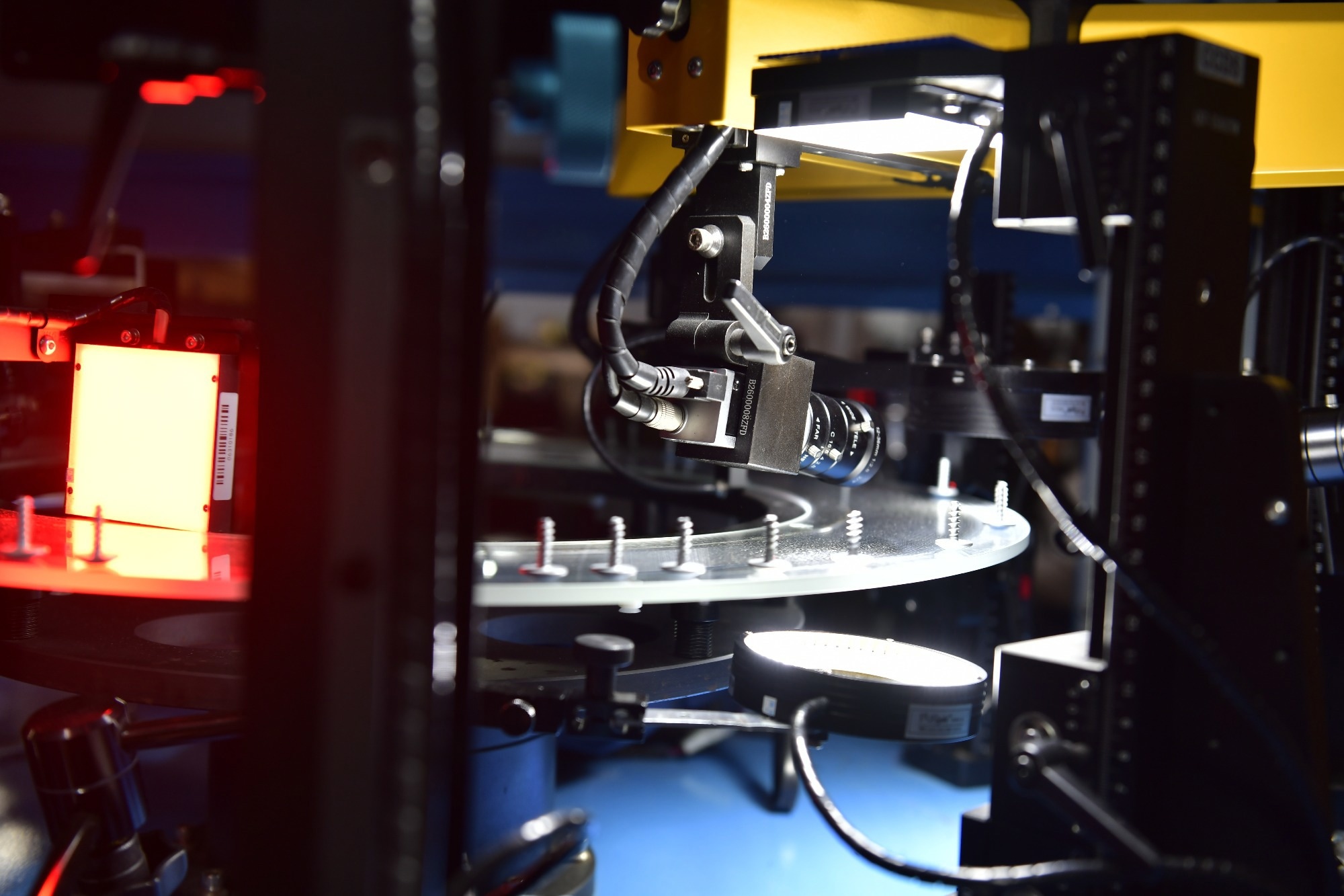 Image Credit: i viewfinder/Shutterstock
History and Definition
The term computational imaging first appeared in the literature in 2003, though the underlying ideas trace back to work on coded apertures for X-ray astronomy in the 1960s. A recent definition frames the field as an image-forming technique that combines optical modulation with substantial algorithmic processing to capture and interpret light-field information.2
A helpful contrast lies in how each paradigm treats a raw sensor frame. Classical photography aims for a picture that already looks correct at the moment of capture. Computational optics accepts a coded measurement that encodes information in a scrambled form, and then recovers the scene through calculation.3
Why did the Field Emerge?
Conventional photoelectric imaging is limited by physical constraints. The Abbe diffraction limit restricts the achievable resolution. Similarly, field of view and resolution are also constrained by each other. Each stage of a camera is built and evaluated in isolation, wasting information that the physics of light has already made available.3
Computational methods relax these constraints by shifting the optimization criterion. Designers stop maximizing energy delivered to a focal plane and start maximizing information transmitted through the entire chain. This reframing allows a reconstructed image to contain detail that a purely optical system of comparable size could never resolve.2
The practical payoff shows up in instrument budgets. A camera built this way can meet a measurement specification with less glass, lower mass, smaller power draw, and reduced cost. Algorithms absorb work that precision manufacturing would otherwise perform, which opens room for optical measurements whose capacity exceeds the physical limits of the optics alone.1
Encoding Light Before Detection
The optical front end in these systems acts as an encoder. Coded apertures, diffractive plates, structured illumination, and programmable modulators deliberately mix scene information across the sensor. Encoding can be active, through controlled light sources and system modulation, or it can exploit how a transmission medium already imprints structure on passing light.3
Using multiple physical dimensions can expand the communication channel. Various parameters such as amplitude, phase, polarization, and spectral content can store distinct information, and a single coded exposure can capture these combinations. Selective acquisition is important in this context. An optimally designed system discards redundant dimensions and allocates measurement resources to essential tasks.3
Randomness serves as an encoder in its own right. Scattering media, diffusers, and disordered surfaces spread light in complex ways that appear destructive. Once the scattering behavior is characterized, that complexity becomes usable structure for imaging through tissue or fog and for non-interferometric phase measurement.4
Decoding Through Algorithms
Reconstruction turns coded measurements back into interpretable results. Iterative solvers, transform-based methods, and trained neural networks all serve this role, and the choice depends on how the optics performed the encoding. Feedback-based optimization pairs the two halves so that decoding matches the specific physics of the capture.1
Recovered output frequently extends past a plain intensity picture. The same raw data can yield depth maps, surface topography, and material properties. Systems built this way also fuse bright-field, dark-field, phase, polarization, spectral, light-field, fluorescence, and volumetric modalities into a single acquisition, providing a fuller description of a specimen.1
Reconstruction quality depends on how faithfully the algorithm models the instrument. Nonlinear image formation, sensor noise, and calibration drift all degrade results when a solver assumes idealized behavior. Careful forward modeling therefore counts as much as the solver itself in determining what the finished system can deliver.3
Metasurfaces give computational optics a compact hardware layer. These ultrathin structures use arrays of subwavelength elements to control amplitude, phase, polarization, and spectral response with precision that bulk glass cannot match at similar thickness. Their ability to manipulate complex light fields directly makes them well suited to the encoding role described earlier.5
Saving this for later? Download a PDF here.
Researchers describe such surfaces as physical preconditioners. The metasurface shapes the wavefront, making the downstream reconstruction problem easier to solve, and the two elements are co-designed through end-to-end inverse design. Automated search over that combined space uncovers surface geometries and reconstruction methods that manual design would likely miss.5
Single-layer designs face a genuine constraint. Packing several functions into a single surface tends to reduce efficiency, limiting how much optical work a thin element can perform on its own. Computational reconstruction compensates for part of that shortfall, so overall system performance stays acceptable even when the hardware layer makes compromises.5
Machine Learning in Optical Design
Differentiable ray tracing allows gradients to flow from a final image metric back to individual lens-surface parameters, such as radii, thicknesses, and aspheric coefficients. A designer can train glass geometry and a reconstruction network together, optimizing both against the quality of the finished output rather than against intermediate optical figures of merit.6
Classical lens optimization stalls at local minima and produces degenerate geometries, such as self-intersecting surfaces, so it usually requires a skilled starting design. A curriculum learning strategy addresses this by beginning with a small aperture and narrow field of view, then raising difficulty in stages while regularization terms suppress unphysical shapes.6
The demonstrated result is an extended-depth-of-field lens in a cellphone-style form factor, designed automatically from randomly initialized flat surfaces, with no human intervention along the way. It holds usable image quality from about 10 cm to 10 m while keeping a large field of view and a small F-number.6
Applications and Open Challenges
Biomedicine has absorbed these methods quickly. Fourier ptychographic microscopy, structured illumination super-resolution, and portable computational microscopes for point-of-care testing and tele-diagnosis all trace back to encode-and-reconstruct thinking. Digital staining driven by machine learning now supplements chemical preparation in some laboratory workflows.1
Beyond the clinic, the same principles support imaging through scattering media, real-time computer-generated holography, security screening, and astronomical observation. Very large aperture systems, bionic optics, and computational detectors represent active research directions, and each of them treats reconstruction as a fixed part of the instrument rather than an afterthought.4
However, there are significant challenges. Nonlinear imaging models resist closed-form treatment, reconstruction demands heavy computation, and performance depends on the optics and software working together correctly. Evaluating such a system requires metrics that assess the combined pipeline rather than the lens alone, fundamentally changing how optical engineers specify and test their work.3
References and Further Reading
- Pan, A. et al. (2024). Computational Imaging: The Next Revolution for Biophotonics and Biomedicine. Cells, 13(5). DOI:10.3390/cells13050433. https://www.mdpi.com/2073-4409/13/5/433
- Liu, J. et al. (2024). Future-proof imaging: computational imaging. Advanced Imaging. DOI:10.3788/AI.2024.20003. https://www.researching.cn/articles/OJe87ae6e3342750d3/html
- Xiang, M. et al. (2024). Computational optical imaging: Challenges, opportunities, new trends, and emerging applications. Frontiers in Imaging, 3, 1336829. DOI:10.3389/fimag.2024.1336829. https://www.frontiersin.org/journals/imaging/articles/10.3389/fimag.2024.1336829/full
- Horisaki, R. (2024). Computational imaging with randomness. Optical Review, 31, 282–289. DOI:10.1007/s10043-024-00881-9. https://link.springer.com/article/10.1007/s10043-024-00881-9
- Roques-Carmes, C. et al. (2025). Metaoptic Computational Imaging. ACS Photonics. 12 (4): 1722–1733. DOI:10.1021/acsphotonics.4c02266. https://arxiv.org/pdf/2411.09133
- Yang, X. et al. (2024). Curriculum learning for ab initio deep learned refractive optics. Nature Communications, 15(1), 6572. DOI:10.1038/s41467-024-50835-7. https://www.nature.com/articles/s41467-024-50835-7
Disclaimer: The views expressed here are those of the author expressed in their private capacity and do not necessarily represent the views of AZoM.com Limited T/A AZoNetwork the owner and operator of this website. This disclaimer forms part of the Terms and conditions of use of this website.