It is often expensive to manufacture and test prototypes in order to verify designs. Also, this may not be practical from a scheduling standpoint. The ability to analyze an opto-mechanical structure then predict the change in wavefront resulting from vibrational loading enables the structure to be optimized without the need to produce costly prototypes.
In the example discussed in this article, a Cassegrain telescope (Figures 1 & 2) was analyzed as it was subjected to a random vibration in a single direction. The Cassegrain telescope is made up of three parts; the primary mirror, the secondary mirror and the mechanical structure which connects the two mirrors. This structure is called the spider.
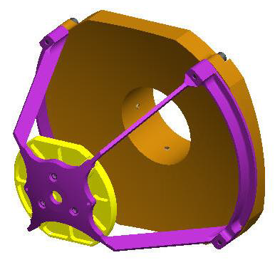
Figure 1. Isometric view of Cassegrain Telescope. Image Credit: Corning Incorporated - Advanced Optics
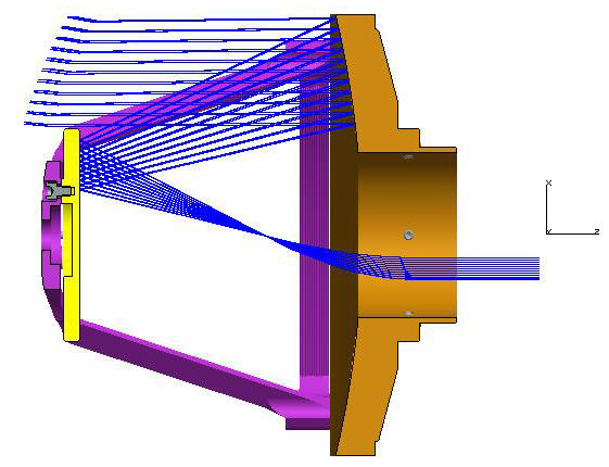
Figure 2. Cross-section view of Cassegrain Telescope showing optical ray trace. Image Credit: Corning Incorporated - Advanced Optics
The random vibration was specified as a provided PSD (Power Spectral Density) function. Two distinct methods were used to analyze the telescope’s secondary mirror - one static and one dynamic - with the results from both analyses compared and contrasted.
Each method employs NX Nastran to undertake a Finite Element Analysis on the telescope. The surface deformations from the FEA were converted to Zernike coefficients using SIGFIT - a software package which is commercially available.
These Zernike coefficients may be applied to the optical surfaces in CODE V® in order to evaluate the effect of the specific disturbance on wavefront.
The Finite Element Model
The finite element model is comprised of a combination of brick elements and parabolic tetrahedron elements. Each of the mirror surfaces is covered with a layer of 2D elements (orange), which are mainly designed for nodal bookkeeping.
The bolted interfaces were estimated with 2X bolt diameter connectivity, while the structure itself is restrained at three different points on the back side of the primary mirror. These points are connected to a single node via rigid elements.
This node was fixed in all six degrees of freedom, for the static analysis. During the dynamic analysis this node represented the vibration source and was fixed in all degrees of freedom aside from one which was oriented in the radial direction (X).
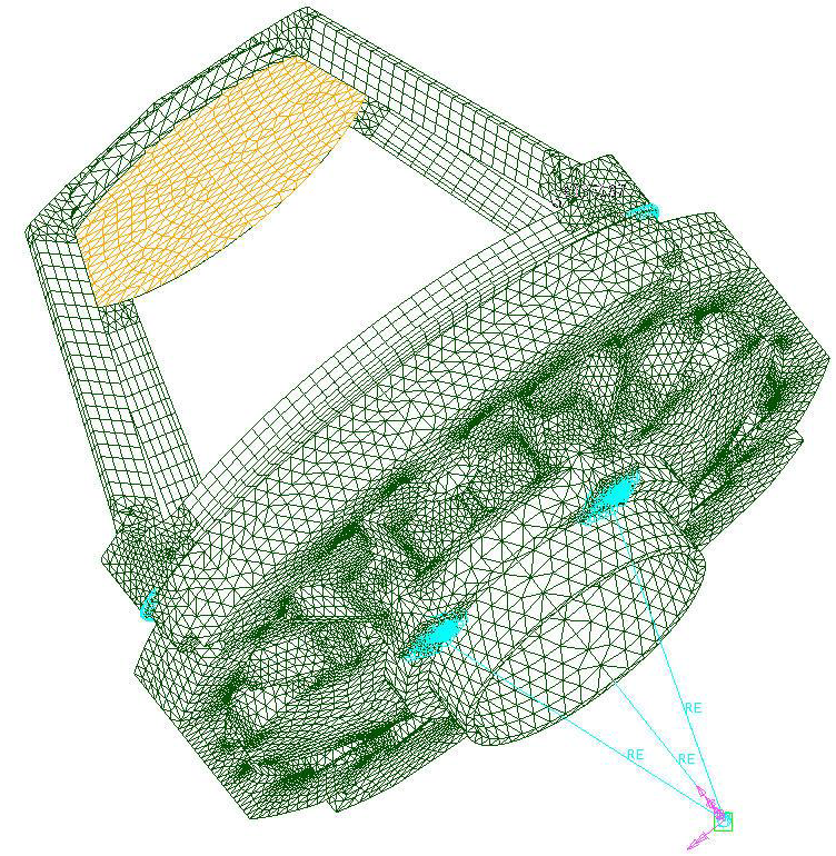
Figure 3. Image Credit: Corning Incorporated - Advanced Optics
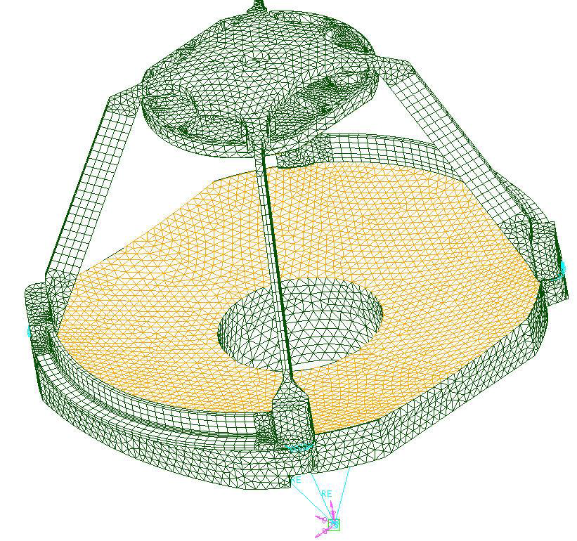
Figure 4. Image Credit: Corning Incorporated - Advanced Optics
Static Analysis
To solve a random vibration issue via static analysis, an equivalent G-load response should be calculated. This involves a number of assumptions: a single degree of freedom system, a random acceleration with a spectrum which is flat in the area of resonance, and being lightly damped.
With these assumptions in place, the following equation was used to ascertain the equivalent static G-load.1
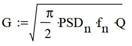
PSD = G2/Hz input at resonance frequency
f = resonance frequency
Q = transmissibility
Here, an FEA model was employed to establish the first three resonant frequencies.
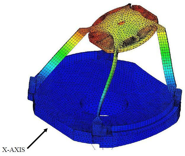
Figure 5. MODE 1 468 Hz. Image Credit: Corning Incorporated - Advanced Optics
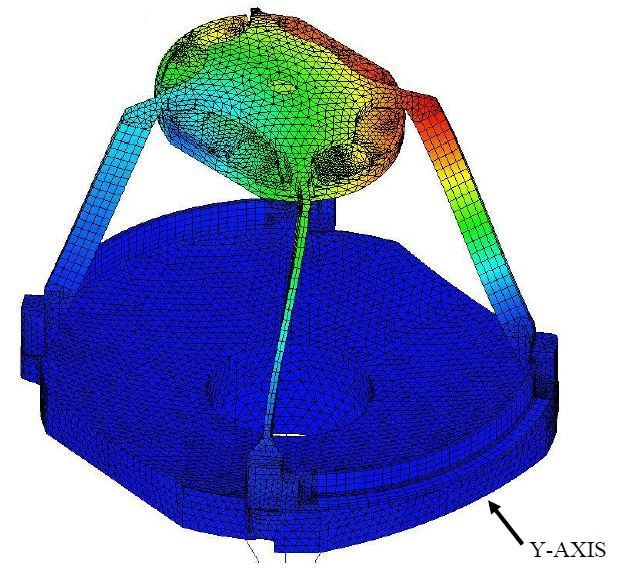
Figure 6. MODE 2 469 Hz. Image Credit: Corning Incorporated - Advanced Optics
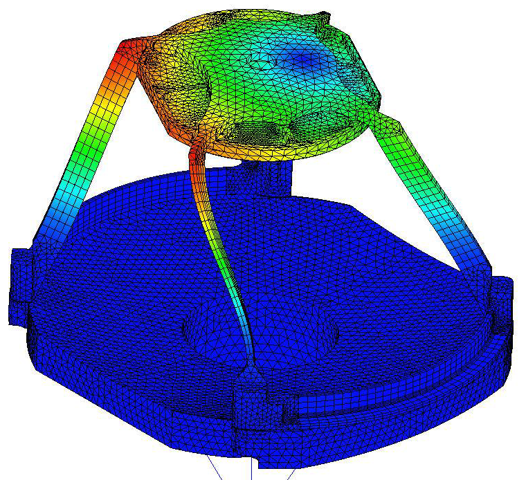
Figure 7. MODE 3 476 Hz. Image Credit: Corning Incorporated - Advanced Optics
Each of these three modes possesses a distinct mode shapes, and each is separated by less than 10 Hz. Within a worst-case example, mode 1 could be employed with the X-direction, thus forcing function since mode 1 is predominately X displacement.
Using the mode 1 resonance frequency value (468 Hz) and the given PSD function (Figure 8) it was possible to determine that the PSD value is .0025 G2/Hz.
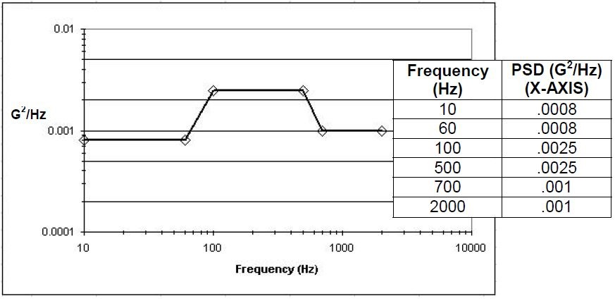
Figure 8. Image Credit: Corning Incorporated - Advanced Optics
The transmissibility (Q) of a lightly damped ‘beam-type’ structure is estimated by inserting the resonant frequency into the following expression:1
Q = 2(ωn)1/2 = 43.27
The equation for the equivalent G-load can now be assessed with the values for PSD, resonant frequency, and transmissibility. This results in a value of 8.9 G’s.
Next, this G-load value was applied to a static FEA, with the load applied in the X-direction. The results of that analysis are displayed in Figure 9.
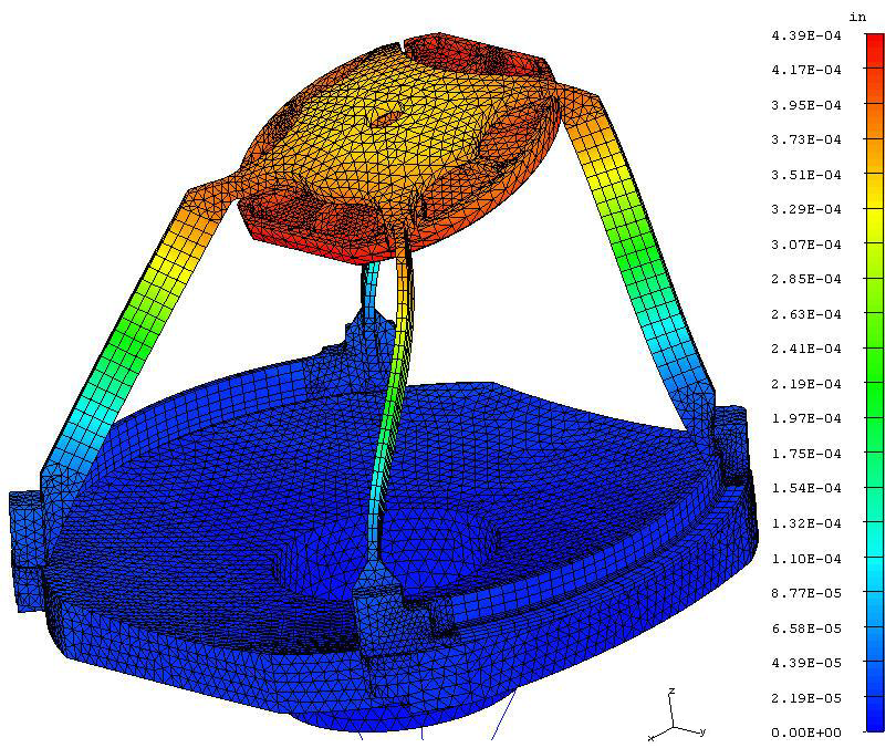
Figure 9. Image Credit: Corning Incorporated - Advanced Optics
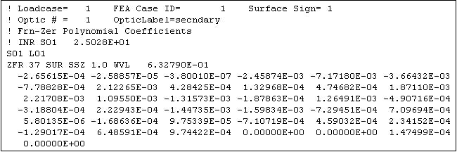
By applying the nodal displacement data gained from the surfaces, SIGFIT was able to perform a fitting analysis which represented the shape of the surface with rigid body motions and Zernike coefficients. Table 1 shows the Zernikes generated for the secondary mirror.
Table 1. Static Analysis Zernike Coefficients. Source: Corning Incorporated - Advanced Optics
These Zernikes were then compared to the results of the random analysis in order to gauge the validity of the static analysis assumptions.
Random Analysis
This example only examines the X-direction, as was done in the static analysis. The first step of the random analysis evaluation is the generation of mode shapes. This modal analysis has similarities with the one undertaken for the static analysis, but has somewhat modified boundary conditions.
A large mass was added to the vibration source node, and this allowed vibration in the X-direction. This node was unconstrained in X. The modal analysis results were identical to the previous static analysis results, with the inclusion of a rigid body mode.
A random analysis was performed by using the modal shape data for the secondary mirror surface along with the PSD table (Figure 8), and also presuming a damping value of 1 percent. This first random analysis was outputted in a modal contribution table.
Table 2. Modal Contribution Table. Source: Corning Incorporated - Advanced Optics
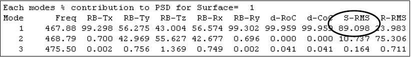
Table 2 displays the modal contributions for the secondary mirror. These include percentage contribution for rigid body motion (RB), for Power (d-RoC) and for surface RMS (S-RMS). These are all with the given PSD. Almost 90 % of the surface RMS is a result of the first mode which justifies the decision to excite in the X-direction. This was done to get the worst-case outcome.
Since the rigid body motion and surface RMS are largely dominated by mode 2’s contribution, a fitting analysis was performed on this mode which represented the secondary mirror surface deformation’s shape. This result proved similar to the analysis performed for the static solution, resulting in the Zernike coefficients shown in Table 3.
Table 3. Random Analysis Mode 1 Zernike Coefficients. Source: Corning Incorporated - Advanced Optics
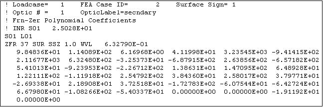
This analysis returns the shape function of the deformed surface, including the removal of rigid body motions. It is important to note that these values are normalized. A surface RMS is calculated based on these normalized values, and was then used to properly scale the Zernikes.
A second random analysis was undertaken using just mode 1 data, allowing a determination of the actual surface RMS contribution from mode 1. This is the value for a one sigma condition, with values not being exceeded 68 % of the time.
It is possible to use these two surface RMS values to calculate a scaling factor.
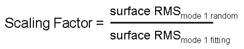
The rigid body motions and Zernike coefficients from the mode 1 random analysis are scaled using this scaling factor. This was done in order to return genuine surface deformations due to mode 1, where the model is excited in the X-direction for one sigma values.
Wavefront aberrations that were created using the rigid body motions and surface irregularities can be evaluated against their specifications. This is the point at which a decision may be made or whether the structure is adequate, or whether it requires appropriate improvements.
Static and Dynamic Solutions Comparison
As the random analysis deformations were dominated by contributions from mode 1, it was anticipated that there would be a degree of correlation between the shape functions returned by each of the two different analyses.
Variations in the magnitude of the rigid body motions and surface RMS were anticipated, because the assumptions used to calculate the equivalent static G-load only loosely fit the criteria for the required assumptions.
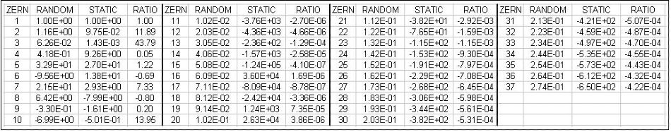
A comparison of shape functions generated by each of the two approaches to analysis highlighted very little correlation (Table 4). Additional investigations are needed in order to fully understand the differences between the two analyses. Because of this, the more rigorous random analysis results should be used to validate optical performance.
Table 4. Zernike Coefficient Comparison. Source: Corning Incorporated - Advanced Optics
Closing the Loop
Mass removal or structural stiffening is required in order to guarantee improvement. A strain energy analysis can highlight regions of the structure which this mass removal or stiffening. After the structure has been modified, the analysis can be repeated to assess the improvements.
Figure 10 shows a strain energy analysis of mode 1.
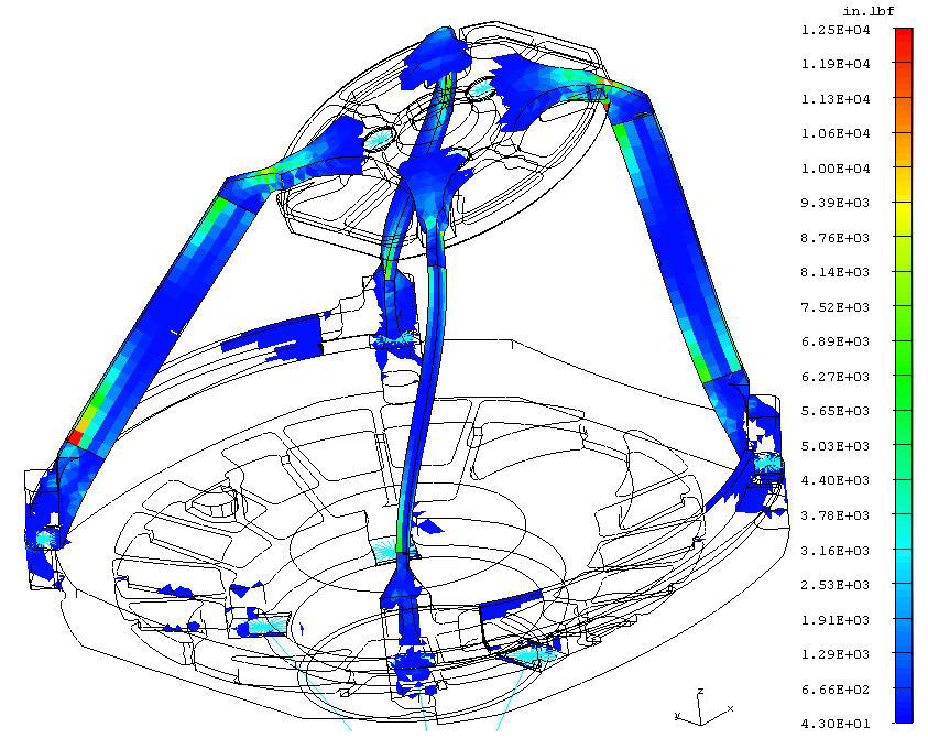
Figure 10. Image Credit: Corning Incorporated - Advanced Optics
Conclusion
The article has demonstrated the way in which mechanical and optical analysis software can be used side by side in order to optimize an opto-mechanical structure which is subjected to vibrational loading.
The output from mechanical analysis software was post-processed into Zernike polynomial coefficients and rigid body motions, before being analyzed with optical modeling software.
Structural improvements can then be implemented where appropriate, based on the results of these analyses.
Within this example, static analysis results failed to match the more thorough random analysis results. This could be because the model’s behavior did not match the assumptions needed for the application of static analysis.
The examples presented within this article are intended to explore the possibility of designing an opto-mechanical structure and optimizing its performance, while avoiding the cost and time implication of working with prototypes.
References
- Steinberg, Dave S., Vibration Analysis for Electronic Equipment, 3rd Edition, John Wiley & Sons, Inc., New York, 2000
Acknowledgments
Produced from materials originally authored by David Bonin and Brian McMaster from Corning Tropel Corporation, with support from Dr. Victor Genberg, PhD and Greg Michels of Sigmadyne.

This information has been sourced, reviewed and adapted from materials provided by Corning Incorporated - Advanced Optics.
For more information on this source, please visit Corning Incorporated - Advanced Optics.