Atomic force microscopy (AFM) is progressively being used to analyze the interactions of lipid bilayers with proteins such as pore-forming toxins (PFTs) and membrane-disrupting peptides.
Image Credit: Elizaveta Galitckaia/Shutterstock.com
AFM can identify protein deployment, heterogeneous protein dispersion in membranes and phase-separated membranes, formation of rings of PFTs, and other structural details relevant for understanding how membrane proteins communicate with cell membranes.
While AFM can provide nanoscale-level structural details of reconstituted PFTs and peptides in membranes, it cannot easily locate the feature of these proteins or detect the extent of dielectric damage caused by PFTs and peptides. Such data is critical in establishing the fundamental relationship between the structure and purpose of biological systems.
For detailed studies of the electrical effects of PFTs in membranes, electrochemical impedance spectroscopy (EIS) is the preferred method. Significant advancements have recently been made in the advancement of EIS data analysis of solid-supported (tethered) phospholipid membranes.
A study, published in Scientific Reports, analyzed the issue of automatic identification of membrane-bound PFTs in AFM images. It was critical to complete this task with sufficient accuracy because the determined coordinates allow users to theoretically measure EIS spectral features and compare them to experimental EIS data.
Researchers introduced a technique for generating synthetic defect sets that resemble detection outcomes of varying accuracy, such as the ones obtained by using an actual object detection model, in addition to applying and checking one of the popular computer vision techniques—convolution neural network.
The current study aims to investigate the potentiality of predicting electrochemical impedance spectra from AFM images of membranes with reconstructed PFTs.
Methodology
Three separate tBLM membrane cells were measured to obtain AFM image data. The assembled tethered lipid bilayers were cultured with vaginolysin for 30 minutes (VLY).
The overall number of annotated deformities and average defect density for each AFM image cell and training/test subset are shown in Table 1. The errors per square micrometer are referred to as defect density. Figure 1 depicts the degree of defect clustering, where higher values correlate to a firmer clustering effect.
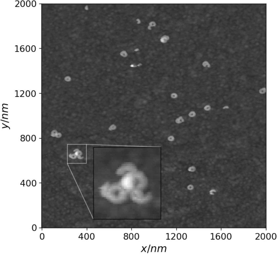
Figure 1. Example of an AFM image fragment with an instance of defect cluster zoomed in. Image Credit: Raila, et al. 2022
Table 1. AFM image sets used for defect detection model training and testing. Source: Raila, et al. 2022
| AFM surface |
Subset |
Image fragments |
N |
Ndef |
σ |
| 1 |
Training |
5 |
202 |
10.10 |
1.18 |
| 2 |
Training |
5 |
138 |
6.90 |
1.12 |
| 3 |
Training |
5 |
170 |
8.50 |
0.77 |
| 1 |
Test |
4 |
172 |
10.75 |
1.20 |
| 2 |
Test |
4 |
97 |
6.06 |
1.02 |
| 3 |
Test |
4 |
158 |
9.88 |
0.91 |
Although the center coordinates and defect radius of membrane deformities are the most important characteristics, these attributes can also be used to convey the deformity position in the image as its bounding rectangle. The accuracy of defect detection can be quantified by correlating two sets of bounding rectangles corresponding to true and expected defect positions.
The bounding rectangle of each true defect position (Btrue) is aligned with its closest prediction to count the number of accurate detections (Bpred). The intersection over union metric (also known as the Jaccard index) evaluates the overlap between each pair of true and predicted bounding rectangles, which is indicated as the ratio of bounding rectangle intersection and union areas in Figure 2.
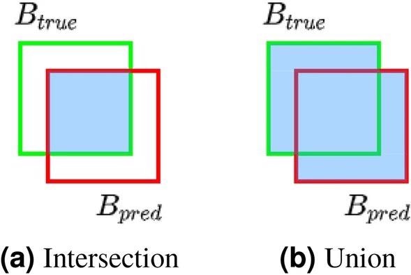
Figure 2. Bounding rectangle overlap of true and predicted defect positions. Image Credit: Raila, et al. 2022
Figure 3 depicts a clustered deformity set and its correlating KDE distribution, where warmer colors coincide with greater probability density function values.
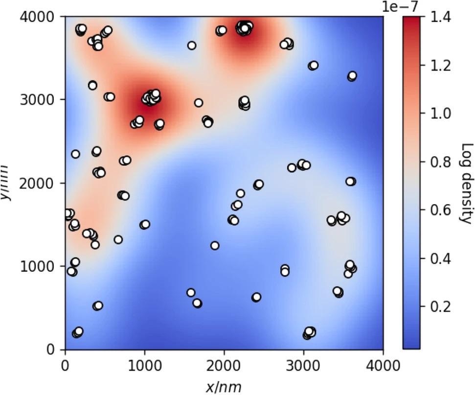
Figure 3. KDE model of true defect coordinates (white dots) annotated for AFM test image #1. Background color represents the log probability density of the fitted KDE distribution. Image Credit: Raila, et al. 2022
The characteristics of the synthetic defect sets obtained by the described procedure are shown in Table 2. Because of the algorithm’s stochastic nature, some clustering variability remains in the defect sets, as illustrated in Figure 4.
Table 2. Summary of generated defect sets for each AFM test image. Precision, recall and F1 values were computed against true defect sets annotated in the given AFM image. Source: Raila, et al. 2022
| AFM surface |
Generated cases |
Precision range |
Recall range |
F1 range |
| 1 |
324 |
0.49 – 1.00 |
0.48 – 0.99 |
0.49 – 0.98 |
| 2 |
256 |
0.54 – 1.00 |
0.51 – 1.00 |
0.53 – 1.00 |
| 3 |
256 |
0.53 – 1.00 |
0.51 – 1.00 |
0.53 – 0.99 |
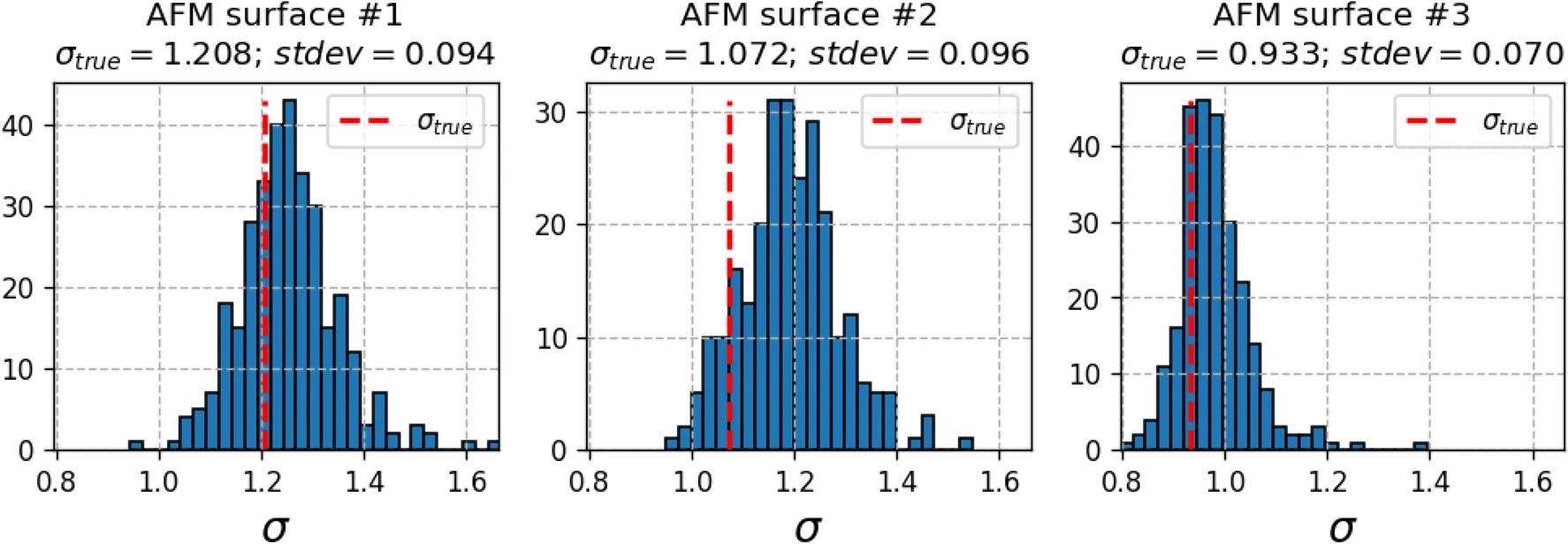
Figure 4. Histograms of standard deviations (σσ) of normalized Voronoi sector areas (multiplied by defect density Ndef) computed for synthetically generated defect distributions. Red dashed lines—Voronoi sector areas of true defect distributions. Image Credit: Raila, et al. 2022
Researchers used the positions of the curves’ minima points along both the frequency and admittance phase axes to measure the difference between the EIS spectra modeled for any pair of true and expected defect sets. Figure 5 depicts the same.
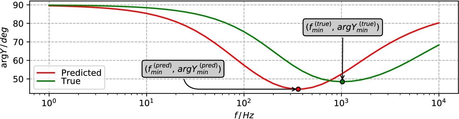
Figure 5. Spectral features of modeled EIS spectra involved in quantifying the difference between true and predicted defect set cases. Image Credit: Raila, et al. 2022
Results and Discussion
A convolution neural network (CNN) model was selected as the present sophisticated approach for object detection methods to conduct the actual defect detection experiments using AFM image data.
Due to the obvious poorly visible surface features within the clusters, defect clusters (Figure 6, left) struggled to resolve. However, for certain image fragments with no defect clusters, the model performed reasonably well (Figure 6, right).
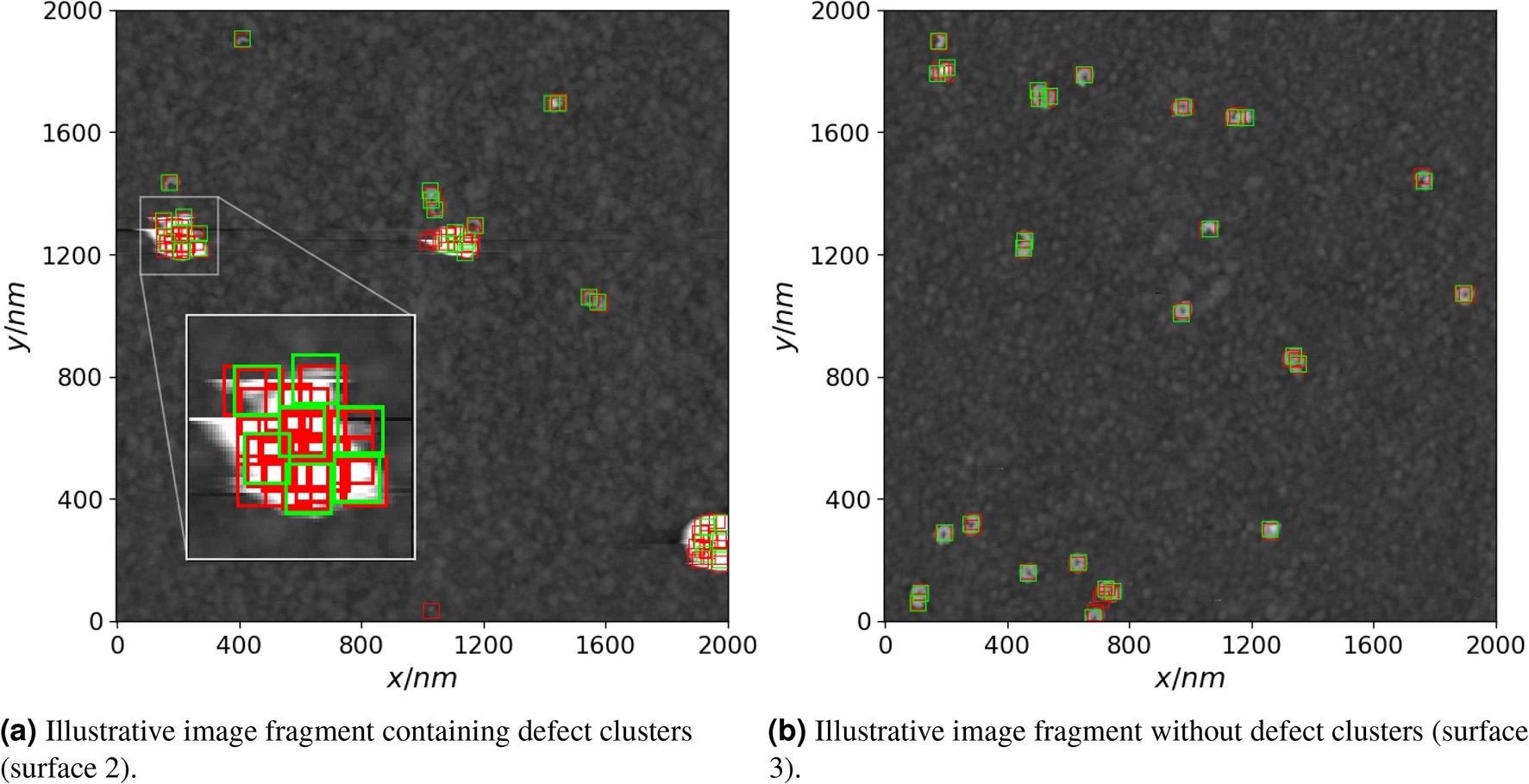
Figure 6. Examples of true defect positions (green rectangles) and predicted (red rectangles) ones by using the convolutional neural network. An instance of a defect cluster and the corresponding true and predicted defect positions is zoomed in on the left image. Image Credit: Raila, et al. 2022
Table 3. Defect detection accuracy of the test AFM images and the resulting differences between EIS spectra of true and predicted defect sets. Source: Raila, et al. 2022
| AFM surface |
Precision |
Recall |
F1 |
QN |
Δ flog |
Δ arg Y |
| 1 |
0.775 |
0.581 |
0.664 |
0.750 |
0.009 |
0.735 |
| 2 |
0.555 |
0.680 |
0.611 |
1.227 |
−0.013 |
0.681 |
| 3 |
0.757 |
0.728 |
0.742 |
0.962 |
−0.027 |
0.864 |
The current AI-based algorithm detects deformities in real AFM images with limited precision. This finding is significant as it suggests that AI-based AFM image analysis can reconstruct EIS spectra with acceptable precision, whereas a mixture of theoretical analysis techniques, EIS, and AI-based AFM image analysis can precisely determine defect densities on real tBLM samples.
To acquire a statistically meaningful approximate of how the precision of an AI-based algorithm may impact the estimation of EIS spectral features, researchers used defect coordinate detection simulation. Figure 7 depicts a graphical summary of the simulation data.
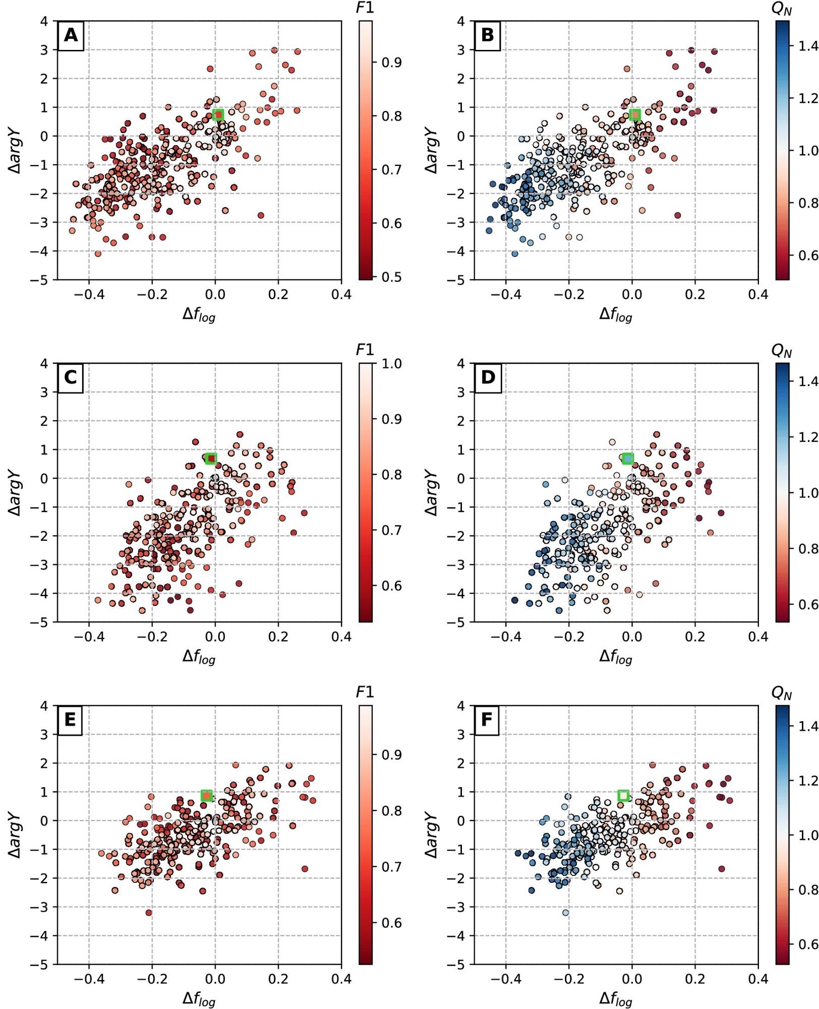
Figure 7. Dependencies between defect detection accuracy (expressed in terms of F1 and QN) and deviations in corresponding EIS spectra. Colored dots represent synthetically generated defect sets at varying detection accuracy levels (Table 2), squares with green borders indicate real detection results obtained with CNN model (Table 3). Scatter plot pairs A/B, C/D and E/F represent AFM surfaces 1, 2 and 3 respectively. Image Credit: Raila, et al. 2022
Figure 8 illustrates the modeled and experimental curves of each surface, as well as the correlating modeled cases’ specific rdef and ρsub values.
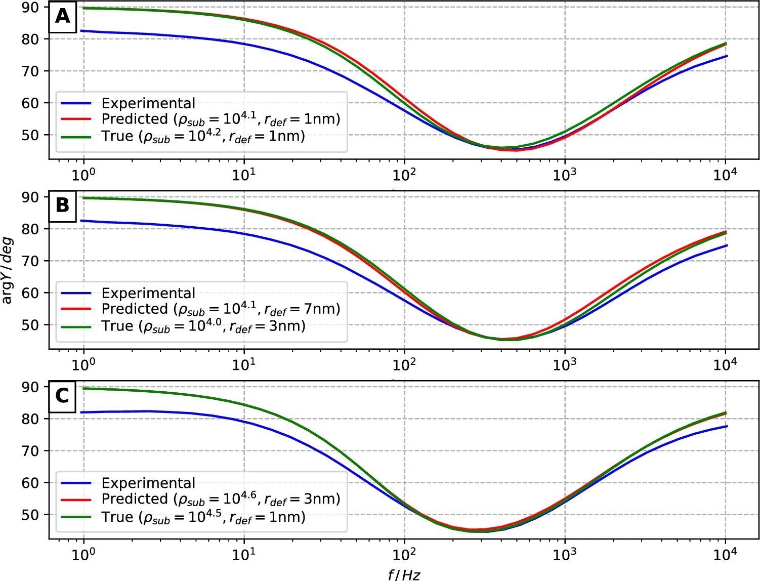
Figure 8. Admittance phase data of experimental EIS measurements (blue curves) versus modeled cases (green and red curves corresponding to manually annotated defect coordinates and CNN model predictions, respectively). (A–C) correspond to AFM surfaces 1, 2, and 3. Image Credit: Raila, et al. 2022
Conclusion
In this study, researchers looked into the potentials of automated defect detection in AFM images of tBLM membranes, as well as the ability to determine the EIS response of such membranes. Researchers also demonstrated the potential advantage of using a convolution neural network for the formulated object detection task over manual defect annotation, though the outcomes should be considered tentative due to a limited number of image data used and the lack of model tuning.
Using three different samples of tBLMs, researchers discovered that, despite being non-identical, true and AI-derived sets of defect coordinates are produced by FEA modeling similar EIS curves.
Finally, researchers show that AFM can be used to evaluate the geometry and composition of membrane-damaging defects such as pore-forming toxins in tBLMs. This data can be used to theoretically predict and calibrate the EIS response of tBLMs for biosensor applications.
Journal Reference:
Raila, T., Penkauskas, T., Ambrulevičius, F., Jankunec, M., Meškauskas, T., Valinčius, G. (2022). AI-based atomic force microscopy image analysis allows predicting electrochemical impedance spectra of defects in tethered bilayer membranes. Scientific Reports, 12(1), pp. 1-11. Available Online: https://www.nature.com/articles/s41598-022-04853-4.
References and Further Reading
- Mulvihill, E., et al. (2018) Mechanism of membrane pore formation by human gasdermin-The EMBO Journal, 37, p. e98321. doi.org/10.15252/embj.201798321.
- Hammond, K., et al. (2021) Atomic force microscopy to elucidate how peptides disrupt membranes. Biochimica et Biophysica Acta (BBA)–Biomembranes, 1863, p. 183447. doi.org/10.1016/j.bbamem.2020.183447.
- Rudd-Schmidt, J., et al. (2019) Lipid order and charge protect killer T cells from accidental death. Nature Communications, 10. doi.org/10.1038/s41467-019-13385-x.
- Richter, R. P., et al. (2006) Formation of solid-supported lipid bilayers: An integrated view. Langmuir, 22, pp. 3497–3505. doi.org/10.1021/la052687c.
- Cornell, B. A., et al. (1997) A biosensor that uses ion-channel switches. Nature, 387, pp. 580–583. doi.org/10.1038/42432.
- McGillivray, D. J., et al. (2007) Molecular-scale structural and functional characterization of sparsely tethered bilayer lipid membranes. Biointerphases, 2, pp. 21–33. doi.org/10.1116/1.2709308.
- Preta, G., et al. (2016) Tethered bilayer membranes as a complementary tool for functional and structural studies: The pyolysin case. Biochimica et Biophysica Acta (BBA)-Biomembranes, p. 1858. doi.org/10.1016/j.bbamem.2016.05.016.
- Valincius, G., et al. (2016) Electrochemical impedance spectroscopy of tethered bilayer membranes: An effect of heterogeneous distribution of defects in membranes. Electrochimica Acta, 222, pp. 904–913. doi.org/10.1016/j.electacta.2016.11.056.
- Raila, T., et al. (2019) Electrochemical impedance of randomly distributed defects in tethered phospholipid bilayers: Finite element analysis. Electrochimica Acta, 299, pp. 863–874. doi.org/10.1016/j.electacta.2018.12.148.
- Raila, T., et al. (2020) Clusters of protein pores in phospholipid bilayer membranes can be identified and characterized by electrochemical impedance spectroscopy. Electrochimica Acta, 364, p. 137179. doi.org/10.1016/j.electacta.2020.137179.
- Tun, T N & Jenkins, A T A (2010) An electrochemical impedance study of the effect of pathogenic bacterial toxins on tethered bilayer lipid membrane. Electrochemistry Communications, 12, pp. 1411–1415. doi.org/10.1016/j.elecom.2010.07.034.
- Valincius, G., et al. (2014) Phospholipid sensors for detection of bacterial pore-forming toxins. ECS Transactions, 64, pp. 117–124. doi.org/10.1149/06401.0117ecst.
- Valincius, G., et al. (2012) Electrochemical impedance spectroscopy of tethered bilayer membranes. Langmuir, 28, pp. 977–990. doi.org/10.1021/la204054g.
- Valincius, G & Mickevicius, M (2015) Tethered phospholipid bilayer membranes. An interpretation of the electrochemical impedance response. Advances in Planar Lipid Bilayers and Liposomes, 21, pp. 27–61. doi.org/10.1016/bs.adplan.2015.01.003.
- Eaton, P & West, P (2010) Atomic Force Microscopy.
- Ewald, M., et al. (2019) High speed atomic force microscopy to investigate the interactions between toxic Aβ1−42 peptides and model membranes in real time: impact of the membrane composition. Nanoscale, 11, pp. 7229–7238. doi.org/10.1039/C8NR08714H.
- Meng, Y., et al. (2018) Automatic detection of particle size distribution by image analysis based on local adaptive canny edge detection and modified circular hough transform. Micron, 106, pp. 34–41. doi.org/10.1016/j.micron.2017.12.002.
- Venkataraman, S., et al. (2006) Automated image analysis of atomic force microscopy images of rotavirus particles. Ultramicroscopy, 106, pp. 829–837. doi.org/10.1016/j.ultramic.2006.01.014.
- Marsh, B., et al. (2018) The Hessian blob algorithm: Precise particle detection in atomic force microscopy imagery. Scientific Reports, 8. doi.org/10.1038/s41598-018-19379-x.
- Sotres, J., et al. (2021) Enabling autonomous scanning probe microscopy imaging of single molecules with deep learning. Nanoscale, 13, pp. 9193–9203. doi.org/10.1039/D1NR01109J.
- Okunev, A. G., et al. (2020) Nanoparticle recognition on scanning probe microscopy images using computer vision and deep learning. Nanomaterials, 10. doi.org/10.3390/nano10071285.
- Sundstrom, A., et al. (2012) Image analysis and length estimation of biomolecules using AFM. IEEE Transactions on Information Technology in Biomedicine, 16. doi.org/10.1109/TITB.2012.2206819.
- Beton, J. G., et al. (2021) TopoStats—A program for automated tracing of biomolecules from AFM images. Methods. doi.org/10.1016/j.ymeth.2021.01.008.
- Hastie, T., et al. (2009) The elements of statistical learning: Data mining, inference, and prediction. In Springer Series in Statistics.
- Scott, D. (2015) Multivariate Density Estimation: Theory, Practice, and Visualization. 2nd edn.
- Lin, T. Y., et al. (2017) Focal loss for dense object detection. In 2017 IEEE International Conference on Computer Vision (ICCV), pp. 2999–3007.
- OpenVINO. SSD ResNet50 V1 FPN COCO. (2021)
- Lin, T. Y., et al. (2014) Microsoft coco: Common objects in context. In Computer Vision—ECCV 2014 (Fleet, D., Pajdla, T., Schiele, B. & Tuytelaars, T. eds.). pp. 740–755.