Self-regulating systems employing feedback loops, i.e., routing the system's output back to its input, have existed since antiquity. These types of systems are now fundamental to modern technology.
James Clark Maxwell’s article, On Governors, documented one of the first attempts to rigorously define control loops that utilize feedback over 150 years ago.1
Regarding control strategies, a controller whose action is determined using predetermined input values without feedback being considered is called an open-loop control system.
Contrastingly, a continuous feedback controller is called a closed-loop control system. This type of controller allows adjustments to be made in real-time to improve precision, stability, and robustness, meaning it is well-suited for achieving the chosen control objectives in changing conditions.
The most widely utilized type of closed-loop control systems are the Proportional–Integral–Derivative (PID) controllers, which constantly measure and adjust a system’s output to match a given setpoint or a target condition for the system or process that is being considered.
PID controllers do not need much prior knowledge or a model of the given system. They are highly versatile controllers, as well as being relatively economical and easy to implement.
This results in PID controllers being used in various systems, including analog and digital electronics, hydraulics, and pneumatics.
They are utilized extensively in various research and industrial applications, such as sensors, photonics, manufacturing, material science, and nanotechnology.
PID control loops are also widely utilized in different aspects of everyday life and industrial automation, including in ovens used for cooking samples or food, gyroscopes employed in self-navigating cars and smartphones, flow controllers used in pipes, and in managing daily vehicle traffic.
However, their presence in more advanced research fields is notable, such as in the following examples:
- Stabilizing laser cavities and interferometers in optics and photonics
- Characterizing mechanical resonators in scanning probe microscopy (SPM)
- Closed-loop controlling of MEMS-based (micro-electromechanical systems) gyroscopes
This article presents PID control loops' main principles and functions by examining their basic building blocks, discussing their strengths and limitations, and outlining the designing and tuning strategies and how they are easy to implement using Zurich Instruments’ lock-in amplifiers.
PID Working Principle and Building Blocks
The purpose of a PID controller is to generate a control signal that enables the dynamic minimization of the difference between the desired setpoint and the output of a given system.
Figure 1 illustrates an exemplary scheme where the first step is the output of the system y(t) being looped back and measured against the setpoint r(t) by the comparator. This produces the time-dependent error signal e(t) = r(t) - y(t).
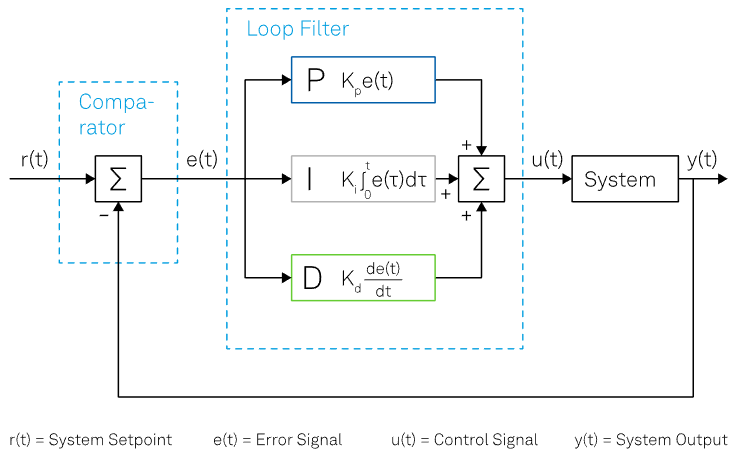
Figure 1. Schematic representation of a general PID control loop in its most general form. Image Credit: Zurich Instruments
The loop filter reduces this error signal and then creates the control signal u(t) that drives the system's output, which is the start of the closed-loop operation. These steps are repeatedly executed to minimize the error.
In addition to the current error, its accumulation over time (represented by the integral) and its future tendency (represented by the derivative at time t) should be considered, as displayed in Figure 2.
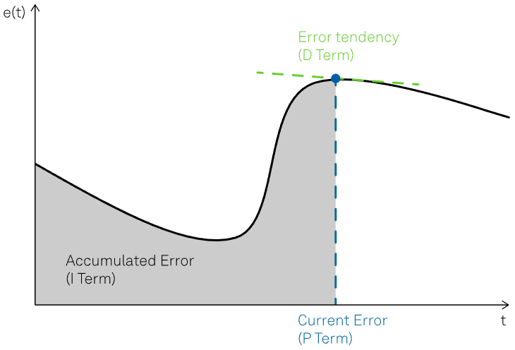
Figure 2. Example of error function with the highlighted contributions of the P, I and D terms. Image Credit: Zurich Instruments
In the most general case, error minimization is realized using the primary components of the PID controller loop filter, namely the proportional term, the integral term, and the derivative term.
Mathematically, the most general form of the complete control function may be written as the sum of the three individual contributions, as follows:
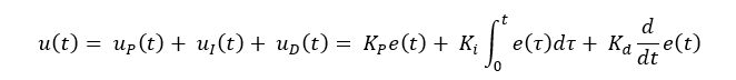
Kp, Ki, and Kd denote the gain coefficients related to the proportional, integral, and derivative terms, respectively.
The Proportional Term
The proportional term is denoted with P. It is based on the current error between the setpoint and the measured output of the system.
This term aids in bringing the system's output back to the setpoint by applying a correction proportional to the amplitude of the error. This reduces the rise time of the correction signal, as depicted in Figure 3.
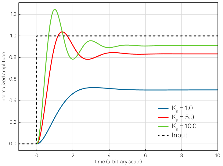
Figure 3. Effect of the proportional action. Increasing the Kp coefficient reduces the rise time, but the error never approaches zero. Additionally, a too high value of the proportional gain might lead to an oscillating output. Image Credit: Zurich Instruments
The larger the error, the larger the correction that is app lied by the proportional term, i.e., the larger the error using a fixed Kp, the larger the value for uP(t).
Since the P term demands a non-zero error to produce its output, it cannot nullify the error by itself. An equilibrium is attained in steady-state system conditions, which includes a steady-state error.
The Integral Term
The integral term is denoted with I. It applies a correction proportional to the time integral of the error (the history of the error). For example, if an error persists over time, the integral term increases, causing a larger correction to be applied to the system's output.
However, the integral term facilitates the generation of a non-zero control signal by the controller, even under a zero-error condition. This allows the controller to bring the system precisely to the desired setpoint, as shown in Figure 4.
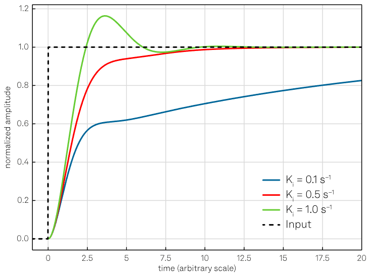
Figure 4. Effect of the integral action with constant Kp = 1. Increasing Ki, the response will be faster but also lead to larger oscillations and overshoot if the value increases too much (green curve). Image Credit: Zurich Instruments
Increasing the integral gain coefficient increases the contribution of the accumulated error over time to the control signal. For instance, if a steady-state error exists, an integral term with a large gain coefficient will drive the control signal to eradicate the error more rapidly than a smaller integral term.
However, too much of an increase in the integral term may result in an oscillating output if too much error accumulates. This leads to the overshooting of the control signal and oscillations being generated around the setpoint. This is a phenomenon sometimes called integral windup.2
The Derivative Term
The derivative term is denoted with D. It provides control over the error tendency (its future behavior) via applying a correction proportional to the time derivative of the error. This enables the rate of change of the error to be minimized, improving the stability and responsiveness of the control loop.
The goal of the term is to predict the changes in the error signal: if the error displays an upward trend, the derivative action aims to compensate without waiting until the error becomes significant (proportional action) or the error persists for some time (integral action).
In real-world applications of PIDs, the derivative action can be omitted because of its high sensitivity to the input signal’s quality.
A rapid change in reference value, e.g., in the case of a very noisy control signal, leads to the derivative of the error often becoming very large. This causes the PID controller to undergo a sudden change that can lead to instabilities or oscillations in the control loop.
Prior low-pass filtering of the error signal is often employed as a mitigation strategy to increase stability. However, derivative control and low-pass filtering neutralize one another, making only a limited amount of filtering possible.
If a derivative term is correctly calibrated and the system is adequately "tolerant", it can result in a derivative action contributing to the controller performance. The effect of the derivative term is illustrated in Figure 5.
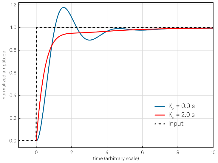
Figure 5. The purpose of the derivative action is to increase the damping of the system; however, too large values of Kd might make the system unstable or oscillatory, as described in the text. The curves are obtained keeping the proportional and integral gain constant (Kp = 4 and Ki = 1 s-1). Image Credit: Zurich Instruments
The effect of each term on the system's response heavily depends on the system's characteristics.
The weighting of the Kp, Ki, and Kd gains may be adjusted to enable the fine-tuning of the control loop’s performance and to achieve the desired responsiveness and accuracy.
Some simple systems or applications may only necessitate one or two of the three control terms offered by a PID controller. In these cases, the controller can be operated using only a subset of these terms by setting the unused terms to zero, providing a PD, PI, P, or I controller.
For example, a PI controller is commonly employed in applications prioritizing steady-state error elimination and stability due to their slow dynamics, compared to rapid response times.
One instance of this is controlling an oven's temperature. In this case, a PI controller is typically employed to guarantee precise temperature regulation and to remove any steady-state offset, considering the relatively slow response characteristics of the oven.
Derivation of an Initial Set of Parameters (Tuning)
A key advantage of PID controllers is the ability to implement them without any knowledge or detailed model of the system.
Heuristic calibration procedures make it feasible to determine coefficients based only on simple experimental tests carried out directly on the process. However, the initial tuning of the PID parameters can still be a delicate task.
There are well-established methods to derive an initial set of coefficients, and several of these involve measuring some of the system’s open-loop parameters.
Open-loop describes a system with no feedback control, meaning that an input signal is applied to the system, and the resulting output is measured, but not fed back to the input.
The input signal may be a ramp, a step function, a sine wave, or any other type appropriate for the considered system.
Subsequently, the system's output is logged as a function of time, and analysis of this can determine the system's response characteristics, including its time constant, natural frequency, and damping ratio.
The typical strategy to identify the initial parameters usually consists of three steps:
- Obtain the open-loop response of the system and measure some of the characteristic parameters, such as the system output’s oscillation period, as well as the process delay.
- Calculate coarse values of the gain coefficients (Kp, Ki, and Kd) utilizing the measured parameters.
- Fine-tune the PID gain coefficients for the optimization of noise, speed, or robustness.
The most widely used techniques to carry out coarse tuning include the Ziegler-Nichols method,3 the Cohen-Coon method,4 the relay method,5 and the Tyreus-Luyben method.6
Table 1 displays an outline example of an initial tuning procedure, created using the Ziegler-Nichols method.
Table 1. Step-by-step procedure for the Initial tuning of a PID controller, based on the Ziegler-Nichols method. Source: Zurich Instruments
| Set the P,I, and D gain to zero |
| ↓ |
| Increase the proportional (P) gain until the system starts to show consistent and stable oscillation. This value is known as the ultimate gain (Ku). |
| ↓ |
| Measure the period of the oscillation (Tu). |
| ↓ |
Depending on the desired type of control loop (P, PI or PID) set the gains to the following values:
| |
Kp |
Ki |
Kd |
| P controller |
0.5 Ku |
0 |
0 |
| PI controller |
0.45 Ku |
0.54 Ku / Tu |
0 |
| PID controller |
0.6 Ku |
1.2 Ku / Tu |
0.075 Ku Tu |
|
| ↓ |
| Test the response of the system and adjust the gains as necessary. If the response is too slow or sluggish, increase the P or I gain. If the response is too fast or oscillatory, decrease the P or I gain. If there is overshoot or ringing, increase the D gain. |
Principles of PID Controllers
References and Further Reading
- Maxwell James Clerk 1868. On governors, Proc. R. Soc. Lond.16270–283
- Y. Tian and D.P. Atherton. Analysis and Design of Reset Control Systems. Institution of Electrical Engineers, 2004.
- Ziegler, J. G., & Nichols, N. B. (1942). Optimum settings for automatic controllers. Transactions of the ASME, 64(6), 759-768.
- Cohen, H., & Coon, G. A. (1953). A linear operator approach to the analysis of closed-loop servomechanisms. Journal of the Franklin Institute, 256(6), 489-512
- Åström, K. J., & Hägglund, T. (1995). PID controllers: Theory, design, and tuning (2nd ed.). Instrument Society of America.
- Luyben, W. L. (1990). Plantwide control: Some practical considerations. Chemical Engineering Progress, 86(4), 49-53.

This information has been sourced, reviewed and adapted from materials provided by Zurich Instruments.
For more information on this source, please visit Zurich Instruments.