Resolution is one of the poorly defined and most often misinterpreted descriptions of performance [1]. The fundamental effects related to aberrations, detector noise, physical optics, the effects of filtering and the role of temporal and spatial bandwidth are some of the few common misconceptions.
Lack of precision in the definition of the term “resolution” is an additional contributor to the confusion. In optical imaging, resolution is defined as the ability to clearly distinguish between closely spaced features or points, usually in accordance with the limits established by physical optics. Resolution is limited by measurement noise or digitization in surface height and distance measuring systems. These two concepts have to be considered independently, for better understanding of the limits of resolution and how to characterize them and perhaps the vocabulary can be adjusted accordingly.
Resolution in 2D and 3D Imaging
Limitations are encountered with densely-sampled images, depending on optical or diffraction quality that restricts the ability of the instrumentation to resolve closely-spaced image features [2]. The presence of two features [3] is still clearly seen owing to lateral resolution, which is the smallest center-to-center separation of features. Figure 1 on the right shows two trenches formed by patterning silicon on a quartz substrate. Although they appear blurred at this high magnification, the interference microscopy 3D image shows that there are in fact two lines present. The optical resolving power of the instrument becomes a constraint in finding out whether the two lines are clearly separated, as the center-to-center separation between the lines decreases.
Cameras with over 5 million pixels are fitted in contemporary laser Fizeau interferometers, offering comprehensive lateral sampling of form, surface texture and waviness [4]. Figure 2 shows the topography image for a diamond-turned disk with a surface height range of a few tens of nanometers. The optical system should be of suitable quality, with huge limiting apertures in order to make the best use of these large-format cameras.
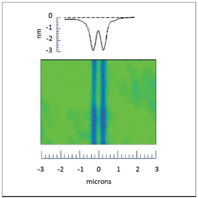
Figure 1. 3D interference microscope image of parallel trenches using a 100x objective with an NA of 0.85. The trenches are 200 nm wide and the center-to-center spacing is 440 nm.
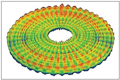
Figure 2. 3D image of a diamond-turned disk using a 100 mm aperture laser Fizeau interferometer.
Quantifying the imaging or lateral resolution of an instrument in terms of a single number, such as the Rayleigh limit [5], is a common practice. Although the specification is more difficult, the modulation transfer function (MTF) and its analog the instrument transfer function (ITF) in 3D metrology offer much extensive information with respect to instrument response as a function of line separation [6].
The response of the system to pure surface sine wave patterns is cataloged by a simple linear ITF as a function of frequency. In the limit of low frequency (<< λ) or small amplitude sine waves, the instrument’s response to the overall surface structure can be predicted by mapping the Fourier components of the surface, weighted by the ITF, to the reported topography [5]. Corresponding closely to the power spectral density (PSD) evaluation of surface error in optical fabrication [7] is a smart feature of the ITF characterization. This literature clearly documents the foundations for a rigorous understanding of the linear ITF and MTF [8]. More complete models permit extending these ideas more normally to larger slopes and steeps in coherence scanning 3D microscopy [9, 10].
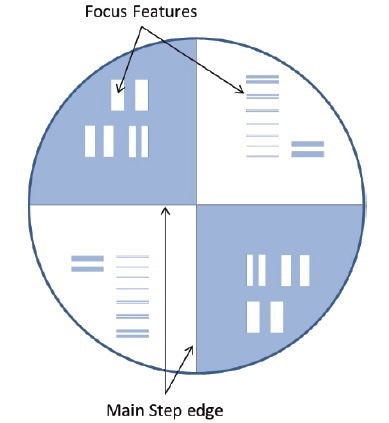
Figure 3. Patterned surface of an ITF measurement specimen with etched features for evaluating the edge spread function.
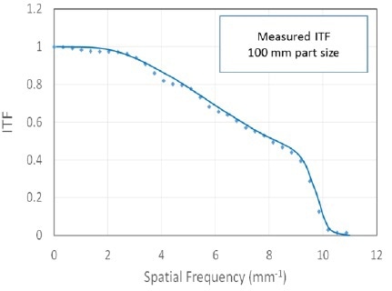
Figure 4. Example precision ITF measurement results showing a design resolution limit of 0.0625 mm or 1600 cycles/aperture.
The 3D equivalent of the edge spread function [11] is used for the ITF measurements, depending on 25 nm sharp step features across the 100 mm full aperture of a super-polished disk. Figure 3 shows that both a vertical and a horizontal edge are present in the test sample, and additional targets are available to enable proper focusing of the instrument. After comparing the frequency content of the measured step to an idealization of a perfect step, the ITF calculation is performed.
An ITF measurement result, in this case for an instrument with a maximum spatial frequency of 16 cycles/mm, is shown in figure 4. To verify that the expected spatial frequency response is uniform across the entire surface area, measurements at different field positions were taken. To prevent camera aliasing [12], the steep slope at high frequencies is consistent with apertures in the intended optical system.
Relating to fundamental physical principles that have little to do with measurement noise is one of the important aspects of imaging resolution. The image shown in Figure 1 can be averaged for a number of days according to one’s wish, and perhaps an extra 10% in resolution can be gained merely from the improved quality of the image. However, there are limitations in the wavelength, the imaging principle and the apertures within the optical system. In the cases of optical coherence tomography and depth discrimination in confocal microscopy, similar constraints are applicable. However, in the following topic, these limits do not apply, at least not in the same way.
Resolution in Distance Measurements
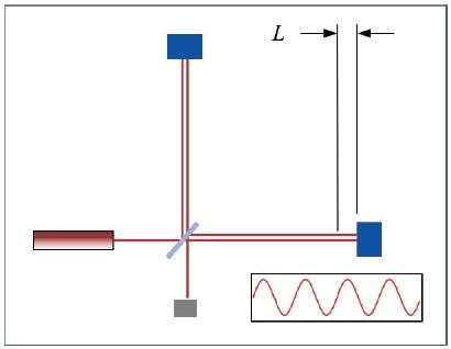
Figure 5. Interferometer for measuring the distance L.
Usually, optical dimensional metrology involves one or more surface height, displacement or distance measurements with respect to a virtual reference plane or point in space. Shown in figure 5 is an interferometric sensor for measuring a displacement or distance L. The smallest detectable change, δL is often called the “resolution”. Unlike imaging resolution, δL which is of significance, is not related to the separation of two object points or distances at the same time. As such, there is no absolute physical limit about how small δL can be. There is no Airy spot with which to contend as a fundamental limit.
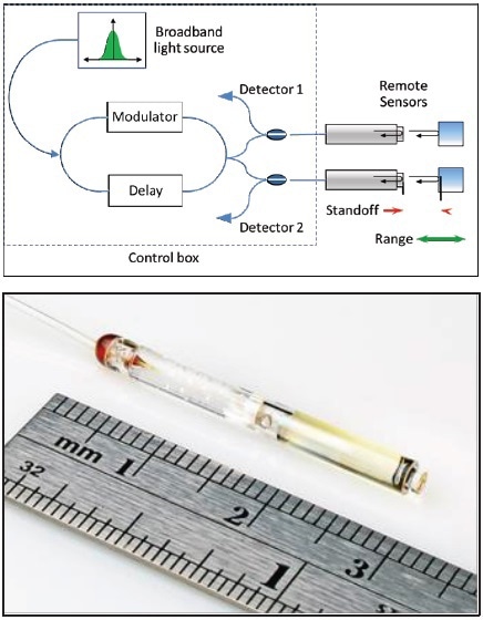
Figure 6. High-precision, fiber-based position sensing system [13, 14].
The “resolution” of distance sensors is synonymous with random measurement noise, assuming that a surplus of digitization is available for recording fine increments. Consequently, proper specification necessarily includes the measurement time or bandwidth [1]. Also with sufficient time, signal to noise and light source power, there is no lower limit to what is achievable in detector sensitivity. Figure 6 shows the contemporary precision sensors such as the fiber-based device. These devices have 3σ noise figures in the 0.5 nm range at 10 kHz, compared to >250 nm limit for the lateral resolution in visual wavelength microscopy.
Table 1. Specifications for the precision sensing system shown in FIGURE 6.
| Fiber sensor specifications [15] |
| Digital Resolution |
0.01 nm |
Noise (3σ) |
0.005 nm/√Hz |
| Data Rate |
Max 208 kHz |
Stability |
1 nm / day |
| Channels |
Up to 64 |
Non-linearity |
± 1 nm |
Resolution in Surface Topography
For the two resolution concepts of interest, areal topography of the surface presents an interesting yet confusing mixture. An array of height measurements over an imaged surface area is provided by interferometers, confocal and focus variation instruments in 3D measuring microscopy. The change in surface height that can be detected is controlled by measurement noise whereas the ability to separate features on the topography map is related to imaging resolution.
It is unfortunate that the term “vertical resolution” is commonly used for such instruments, as it leads to confusion of the two concepts. This is clear in specification sheets for these instruments, which, with few exceptions, make no mention of time bandwidth or measurement speed when quoting vertical resolution [16]. Draft ISO standards for calibration will probably command a correction to this practice [17].
Regions Analysis with Mx Software, Part 1: Optical Profiler Surface Topography Measurement
3D interference microscopes remain diffraction limited apart from model-based techniques comparable to scatterometry and enhancements to image clarity and correction for undersampling. On the other hand, surface height “resolution” has the scope to advance, depending on data acquisition speed, camera pixel count and quantum well depth. The present state of the art for interference microscopy, for instance, offers better than 0.1 nm √Hz over one million height measurements taken at the same time [18]. Following the familiar √N rule means that in 100 seconds, 10 pm repeatability is achieved. It is advisable to think about enabling technologies and methods that can reduce this even further without altering any fundamental limits.
The Limits of Resolution
To characterize the limits of resolution requires an adjustment in our vocabulary. It would be preferable in technical reports and specification sheets to reserve “resolution” for those metrology attributes that are restricted by user’s ability to noticeably separate surface depths or neighboring features as in 3D and 2D imaging. It would be better to quantify the measurement noise or the equivalent, for distance measurements, including height measurements for widely-separated surface features, carefully observing if it is a single standard deviation or a multiple thereof.
There is a wide range of useful characterization techniques, once the common language is spoken. In the case of imaging resolution, depending on the edge spread function and other techniques, sample specimens with closely-spaced features complement linear ITF techniques. The corresponding noise levels, for distance measurements, can often be determined from repeatability tests over a range of bandwidths. These characterization methods allow for sensible comparison of advances in performance, instrumentation and adaption of measurement methods to demanding applications.
Acknowledgements
The Authors recognize the contributions of ZYGO Scientists and Engineers to the results shown in this paper. We also thank Prof. Richard Leach for his review of the draft manuscript.
References
[1] Understanding Sensor Resolution Specifications and Performance. Lion Precision TechNote. 2014:
[2] de Villiers, G., and Pike, E. R. The limits of resolutoin. CRC Press, Boca Raton, 2017.
[3] ISO DIS 25178-600:201: Geometrical product specifications (GPS) - Surface texture: Areal - Part 600: Metrological characteristics for areal-topography measuring methods (DRAFT 2017-03-29) International Organization for Standardization, Geneva 2017.
[4] Sykora, D. M., and de Groot, P., Instantaneous measurement Fizeau interferometer with high spatial resolution. in Optical Manufacturing and Testing IX, Proc. SPIE. 2011; 8126: 812610-812610-10.
[5] de Groot, P., Colonna de Lega, X., Sykora, D. M. et al. The Meaning and Measure of Lateral Resolution for Surface Profiling Interferometers. Optics and Photonics News. 2012; 23: 10-13.
[6] de Groot, P., and Colonna de Lega, X., Interpreting interferometric height measurements using the instrument transfer function. in 5th International Workshop on Advanced Optical Metrology, Proc. FRINGE Springer Verlag. 2006; 30-37.
[7] ISO 10110-8:2010(en), Optics and Photonics – Preparation of drawings for optical elements and systems International Organization for Standardization, Geneva 2010.
[8] Goodman, J. W. Introduction to Fourier Optics. McGraw-Hill, New York, 1996.
[9] Coupland, J., Mandal, R., Palodhi, K. et al. Coherence scanning interferometry: linear theory of surface measurement. Applied Optics. 2013; 52: 3662-3670.
[10] Su, R., Wang, Y., Coupland, J. et al. On tilt and curvature dependent errors and the calibration of coherence scanning interferometry. Optics Express. 2017; 25: 3297-3310.
[11] Takacs, P. Z., Li, M. X., Furenlid, K. et al. Step-height standard for surface-profiler calibration. Proc. SPIE, 1993; 1995: 235-244.
[12] Deck, L. L. Method and apparatus for optimizing the optical performance of interferometers. US patent number Application 15/383,019. 2016.
[13] Badami, V. G., Wesley, A. D., and Selberg, L. A., A high-accuracy, multi-channel, fiber-based displacement/ distance measuring interferometer system. in Annual Meeting of the American Society for Precision Engineering, Proc. ASPE ASPE. 2013;
[14] de Groot, P., Deck, L. L., and Zanoni, C. Interferometer system for monitoring an object. US patent number 7,636,166. 2009.
[16] de Groot, P., The meaning and measure of vertical resolution in surface metrology. in 5th International Conference on Surface Metrology, Proc. ICSM. 2016;
[17] ISO WD 25178-700.2: Geometrical product specifications (GPS) - Surface texture: Areal - Part 700: Calibration and verification of areal topography measuring instruments (DRAFT) International Organization for Standardization, Geneva 2017.
[18] Fay, M. F., Colonna de Lega, X., and de Groot, P., Measuring high-slope and super-smooth optics with high-dynamic-range coherence scanning interferometry. in Optical Fabrication and Testing (OF&T), Classical Optics 2014, OSA Technical Digest. 2014; paper OW1B.3.

This information has been sourced, reviewed and adapted from materials provided by Zygo Corporation.
For more information on this source, please visit Zygo Corporation.