Structural damage in components is frequently not apparent from the outside. However, ultrasonic waves can be utilized for Structural Health Monitoring (SHM). The propagation of waves and their interaction with defects can be analyzed and reported in a full-surface, high-precision, and contactless manner by employing scanning laser vibrometry.
This article briefly outlines the theories of the ultrasonic waves utilized, known as Lamb waves, along with 3D scanning laser vibrometry. The key section of the article shows measurement results acquired using this technique featuring both the propagation of waves and their interaction with defects.
Lamb Waves for Defect Identification
The scanning of plates or panels using ultrasonic transducers is a common technique for detection of defects in safety critical components.
This method commonly requires that the receiver and transmitter are on opposite sides of the panel. Alternatively, with the ‘back-wall echo method’, they are on the same side with transducers coupled to the panel, for example by utilizing water, which in the majority of cases is a limitation.
Another method observes propagating guided waves in the panel and their interaction with defects.
Thin-walled load-bearing components were almost always made from sheet metal in the past, but today are increasingly made from carbon fiber reinforced plastic (CFRP) panels . These waves propagate as compression waves and flexural waves within the plate.
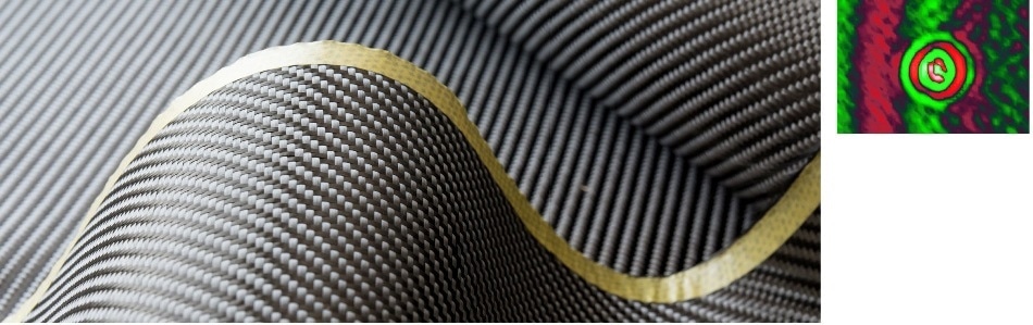
Figure 1. Mode conversion from symmetric and asymmetric Lamb waves at a structural defect.
Figure 2 shows a cross-section through groups of compression and flexural waves in aluminum (actual measured data). No matter whether structural damage or a material defect is located on an inaccessible face or in the center of the material, a wave, which can be observed from the accessible face, interacts with it and exhibits modified behavior.
One way to monitor defects during actual use in the field (such as in panels during flight), is to install piezo-based sensor-actuator networks.
The sensor signals can be employed to establish the state of the component. The only way to gain insight into the complicated physical processes and to accurately assess these point measured signals is to constantly observe the behavior of the waves over space and time in the research and development phase.
Scanning laser vibrometry can easily and effectively achieve this. Moreover, current vibration amplitudes in the high tens of nanometer range and excitation frequencies up to several hundred kilohertz can be reached with ease.
Scanning laser vibrometry is also highly appropriate for the layout of these kinds of piezo-sensor networks. Additionally, it provides an independent technique for defect detection, in cases where conventional ultrasonic transducer methods are impractical.
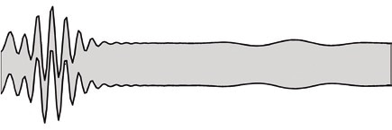
Figure 2. Compression and flexural waves in aluminum sheet over 250 mm, true sheet thickness 1 mm, true vibration amplitudes less than 100 nm.
3D Scanning Laser Vibrometry
A 3D Scanning Vibrometer is a measuring system for the interference-free and contactless analysis of 3D vibrations in mechanical structures.
The technique is founded on the optical Doppler effect, which makes light waves scattered from moving surfaces to develop a variation in frequency, where the change is related to the movement.
The frequency change is directly proportional to the simultaneous value of the vibration velocity. In spite of its incredibly small relative value of less than 10-8, it can be accurately calculated employing interferometric methods.
Inside the vibrometer, for this purpose, the back-scattered laser light is compared to a reference beam whose frequency has been adjusted by a determined amount (the heterodyne process, shown in Figure 3).
The velocity component in the beam direction has an influence on the Doppler frequency shift only. A 3D Scanning Vibrometer (Figure 4) is consequently employed to fully measure the velocity vector at the measuring point.
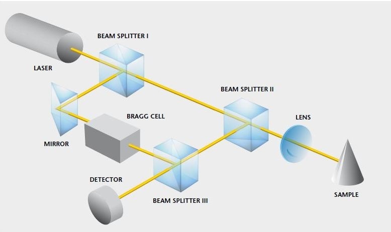
Figure 3. Optical design of a laser vibrometer.
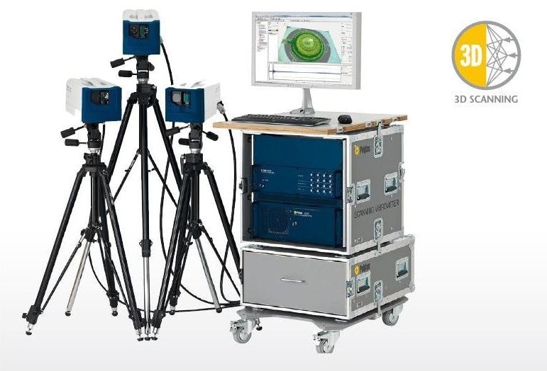
Figure 4. A 3D Scanning Vibrometer for full-field measurement to measure both out-of-plane and in-plane motions.
It utilizes three differently oriented and independent laser beams to completely record the movement of each measurement point. Along with the standard FFT vibration analysis mode, it is also a possibility for wave monitoring to analyze in the time domain.
If experimental repeatability can be ensured, the same burst signal is applied to the actuator to excite waves for every point of the scanning grid and is then repeated for each point.
To ensure that distinct measurements are properly synchronized with each other, the time interval between the start of measurement and excitation must be triggered in the exact same way each time, causing no transfer functions. The storage and capture of a reference signal is not completely important in this case.
The area is segmented by the scanning grid in laser vibrometry, while the time signal is recorded almost constantly.
As such, this method is fundamentally different from, for example, holography and ESPI (electronic speckle pattern interferometry), where the area is analyzed quasi-continuously over the observed surface, but the time is measured in discrete steps.
A single set-up process is adequate to allow for the complete acquisition of the data record in terms of position and time through automated scanning.
1D Scanning Laser Vibrometry: Observation of Oblique Vibrations
1D scanning systems demand one-dimensional vibrations in the direction of the non-deflected laser axis (normally the z-axis). In this event, the velocity vector of a scan point solely has component vz = v (shown in Figure 5, left).
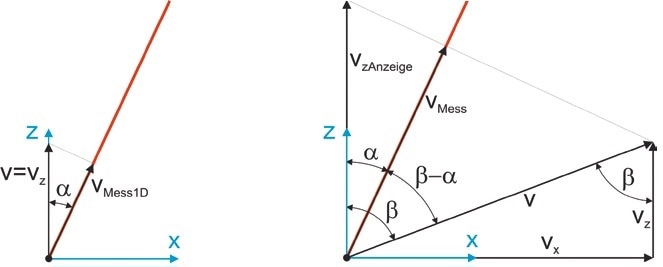
Figure 5. Velocity vector of a scan point and geometric conditions of the deflected laser beam (left: one-dimensional vibration, right: multidimensional vibration).
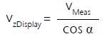
Fundamentally, vibrometers analyze the velocity component in the direction of the laser axis, so that the measured variable vMeas1D is divided by the cosine of the deflection angle α to acquire the vibration velocity vz :
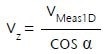
In the case of Lamb waves where the vibrations are no longer one-dimensional in the z-direction, this cannot be compensated by the angle correction capability of the Polytec Scanning Vibrometer software.
The velocity vector v of a scan point is then rotated away from the z-axis by the angle α. The detected vibration by the vibrometer is also the component parallel to the laser axis, in this example vMeas.
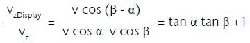
To the right of Figure 5, the geometric relationships are indicated:
vMeas = v cos (β - α)
Using the equation:
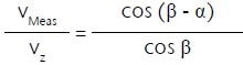
The angle correction capability of the PSV software corrects the laser’s deflection angle. In adherence to the Cartesian decomposition of v, the z component is:
vz = v cos β
As such, the error factor is:
Consequently, if a pure z-vibration happens (β = 0) or if the laser beam is precisely perpendicular to the surface (α = 0), there is no error. If at least a single angle approaches 90°, the error becomes infinite. The laser can be pivoted through 20° about each of two spatial axes in PSV systems, so that subsequently a maximum angle α = tan–1 (√2 tan 20º) = 27,24º is the result.
In Figure 6, the error factor recorded is marked in blue for the valid α range for different values of β (0°, 22,5°, 45°, 67,5°, 80°, 89°).
Additionally, the error factor as a result of the angle correction being deactivated in the data acquisition software is shown in red. Only for β = 0° does this cause an error factor < 1, or else the error is slightly smaller than when angle correction is activated. Although, a quantitative analysis of the data continues to be invalid.
The error has a beneficial effect on purely qualitative investigations utilizing 1D vibrometers where it enhances the signal-to-noise ratio of the out-of-plane amplitudes of symmetric Lamb waves. However, quantitative studies demand a 3D measurement system, or they can only be carried out at points where the laser beam is directed in a normal fashion to the surface.
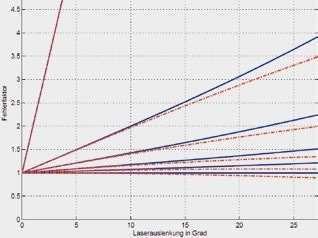
Figure 6. Error factor for out-of-plane amplitudes throughout 1D scanning of oblique vibrations: β = 0°, 22.5°, 45°, 67.5°, 80°, 89° (increasing gradient) for active (blue) and deactivated angle correction (red).
Ultrasonic Waves in Plates Theory of Lamb Waves
As mentioned before, waves in plates generate as compression and flexural waves (in-plane shear waves are not included here). In 1917, Horace Lamb1 was the first person to find an analytical solution to the Navier-Lamé differential equation
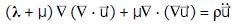
for an isotropic, homogeneous, and ideally elastic continuum bounded by two planar surfaces. For example, intended for waves in a metal plate or sheet. The solution is known as the Rayleigh-Lamb frequency equation,
are the known Lamé constants (to be determined from Poisson’s ratio and Young’s modulus) and ρ is the density of the material, providing information about the behavior of dispersion, that is the frequency dependence of the phase velocity c, of the waves under observation along with their multi-modality.
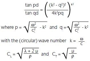
There are at least two solutions to the equation for each excitation frequency, and therefore at least two wave modes. The first two solutions are called fundamental modes, S0 und A0, and occur for each ƒ respectively ω > 0. They are demonstrated in the numerical assessment of the equation shown in Figure 7 as the bold curves.
The solid lines signify the phase velocities of symmetric Lamb waves (compression waves), which were determined using the equation with the exponent equal to +1, the asymmetric modes (flexural waves) are represented as dashed lines determined with the exponent equal to -1.
In the representation of such dispersion diagrams, it is traditional (as done here) to apply phase velocities using the frequency-thickness product of the plate, so that a diagram is valid for any plate thickness.
A more detailed description of the theory of Lamb waves can be located in Structural Health Monitoring by Victor Giurgiutiu2.
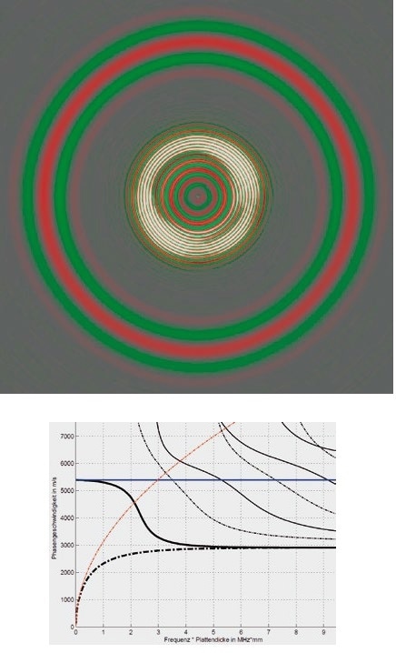
Figure 7. Above: Propagation of symmetric (outer) and antisymmetric (inner) Lamb waves in an aluminum plate. Below: Dispersion of Lamb waves in an aluminum plate. (Solid lines: symmetric modes, dashed lines: anti-symmetric modes, bold: fundamental modes. Blue: Compression waves according to assumption of plane stress, Red: flexural waves according to Kirchhoff theory).
1 Sir Horace Lamb, English mathematician and physicist, 29.11.1849 – 4.12.1934
2 Giurgiutiu, Victor: Structural Health Monitoring with piezoelectric wafer active sensors
Along with the precise description of Lamb waves founded on the mathematics of continuum mechanics, flexural and compression wave features can also be determined from simplified plate theories.
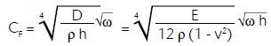
At low frequencies, the results acquired in this method are the same as those found using Lamb wave theory. Although, at higher frequencies, the simplifications result in significant errors. The non-dispersive plate compression wave velocity (red curve) from the assumption of plane stress
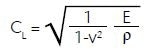
relates to the S0 phase velocity, and the flexural wave velocity (blue curve) derived from Kirchhoff plate theory
relates to the A0 phase velocity. The diagram signifies deviation and overlap areas. Figure 7 detailed above exhibits the out-of-plane displacement field from a 1D measurement of Lamb waves (S0 and A0 modes) in an aluminum plate after a burst excitation from a piezoceramic actuator in the center.
Theory of Ultrasonic Waves in Composite Fiber Panels
Lamb wave theory is only applicable with the following limitations:
- isotropy,
- homogeneity, and
- ideal elasticity.
A good estimation to ideal elasticity can be inferred (in the technically relevant frequency range) for fiber-plastic composites established on thermoset matrix materials. This simplification cannot be inferred for materials with greater internal damping. Homogeneity is as unsuitable to fiber composites as isotropy.
The anisotropy of the elasticity parameters creates deviations of the wave fronts from the circular to different degrees. Numerical calculation techniques for example the finite element method can quickly become limited in the estimation of the propagation and interaction behavior of waves.
Realistic modeling of individual carbon fibers would incur unacceptably high costs. However, each simplification demands experimental validation of its replace admissibility with acceptability. As such, measurements are critical for modeling the propagation of Lamb waves.
Figure 8 demonstrates a common example of the propagation of a compression wave (S0 Lamb wave) in a highly anisotropic composite fiber panel. The data record was gathered utilizing a 1D Scanning Vibrometer. A sinusoidal burst signal applied to a piezoceramic actuator in the center of the panel caused the excitation of the wave.
As there is a difference in the phase velocity of the two fundamental wave modes excited in this method, the wave groups are isolated from each other and can be observed individually. The middle is recessed as a result of the amplitude increase in the proximity of the actuator.
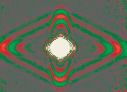
Figure 8. Propagation of compression waves in a highly anisotropic carbon fiber reinforced plastic panel.
3D Scanning Vibrometry for Wave Observation
The vibration amplitudes for Lamb waves are tiny, only a few hundred nanometers at wavelengths in the millimeter to two-figure centimeter range. The amplitudes are presented (Figure 9) with a greatly magnified height in order to simply visualize the waves.
This kind of spatial visualization is no challenge for 1D measured data. Although, due to spatial movement and significant in-plane components, the movement trajectories of alternately vibrating points in the animation can overlap with each other and may therefore suggest a false distortion profile.
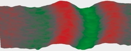
Figure 9. Symmetrical (compression) wave fronts with a highly magnified amplitude from a 1D measurement.
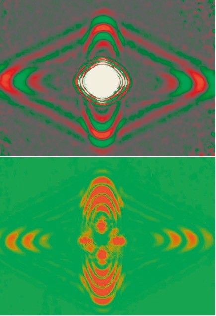
Figure 10. 1D (out-of-plane, left) and 3D measured data (all three movement components x, y and z, right) of compression waves in an anisotropic panel.
As such, it is advised to evaluate the data acquired from 3D scans either through the use of the color palette, thereby largely forgoing the geometric animation, or to visualize the three vibration directions individually as 1D representations.
Figure 10 similarly demonstrates the propagation of symmetric waves in an anisotropic plate from Figure 8. However, this time the results are presented in contrast to each other as 1D (left) and 3D measurements (right).
The images portray the same section of the same experiment. Although, in 3D representation space, the software generally cannot allocate an unambiguous sign and as such the color palette only extends over the unsigned amplitude contributions.
Green and red signify negative and positive amplitudes on the left, while on the right, green means stationary and red signifies a high amplitude of any sign.
Moreover, on the right, the wavelength seems to be halved, which must be included in the assessment. In the following, all 1D representations are illustrated in green-black-red and all multidimensional representations are portrayed in green-red.
In experiments on (flat) CFRP panels, the apparent solution is to determine the measuring surface in the x-y plane and to align the x- and y-axes of the Cartesian coordinate system of the software with the main axes of the panel under test, as was performed in the current case. Therefore, the in-plane and out-of-plane amplitude components are displayed in a convenient manner.
Figure 11 categorizes the experiment into its movement components:
- In-plane, x component
- In-plane, y component
- Out-of-plane, z component
- In-plane, x-y component
It is clear that the compression waves mostly create vibrations in the plane of the plate and in this regard, the most important fraction of the vibrations happen in the propagation direction. Only light shadows can be identified for the same scale in out-of-plane vibration.
The antisymmetric flexural waves, propagating more slowly, can be observed in the middle of the plate in the z-amplitudes. Its movement fraction is more out-of-plane than in-plane.
Although, this statement is only correct up to specific limiting frequencies in which the actual situation is reversed and is angularly dependent in anisotropic materials. The ratio of bending to longitudinal stiffness of the plate, both directional and anisotropic values, have an impact on the cut-off frequency.
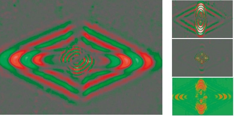
Figure 11. Compression waves in an anisotropic panel: Amplitudes in the x (left), y (above), z (center), and x+y direction (below).
Detection of Structural Damage Caused by Wave Interaction
As discussed in the introduction, material errors and structural damage are often hard to distinguish. A significant example is impact damage to CFRP structures, which commonly manifests as delamination, such as the detachment of distinct laminate layers from one another.
Damage Detection Experiment
3D measurements are performed on an undamaged, quasi-isotropically laminated CFRP panel to collect reference data. The excitation is generated by a sine-windowed burst signal 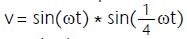 of two sine wave periods in length applied to a piezoceramic wafer, with the measurements being performed in the time domain.
Figure 12 demonstrates the signal and its amplitude spectrum. The application of the window decreases the undesired secondary maxima in the spectrum. The experiment is repeated for various excitation frequencies.
At first, a group of compression waves moves through the area of observation, subsequently, due to the lower phase velocity, a group of flexural waves pass through.
To create a location of impact damage, a drop hammer with a kinetic energy of 2.5 J and a circular impact area of 12.5 mm2 (shown in Figure 13, above) strikes the back side of the panel. This creates a surface impression of 0.05 mm in depth (Figure 13, below).
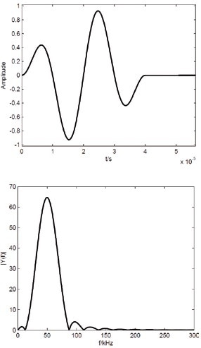
Figure 12. Excitation signal in the time domain (upper) and related amplitude spectrum (lower).
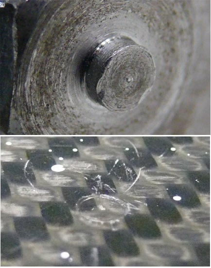
Figure 13. Above: Front face of the drop hammer Below: Impression after the 2.5 J impact.
Under the same conditions, the measurements were repeated after the damage. Figure 14 portrays a snapshot of the out-of-plane velocity field in the observation area prior to (above) and after (below) the impact event.
As an example, a 50 kHz excitation was utilized. In the lower snapshot, the defect is slightly distinguishable because of the circular secondary waves. The difference between the two data records is imaged utilizing the signal processor (software option PSV 8.7 or higher) or by using MATLAB.
The left of Figure 15 shows only the out-of-plane components; at center, only the in-plane components; and, at right, all the vibration directions at once. The difference data provides a visible indication of the position of the structural damage. It is also clearly observed that out-of-plane vibrations provide much clearer results compared to in-plane vibrations.
What is not apparent from the still photos is the fact that the passing of the primary S0 -group (Figure 16, left), and also the consequent passing of the A0 -group (Figure 16, right), gives rise to new flexural waves developing around the damage. Despite this, the difference image (Figure 15) presents greater secondary waves for the primary A0 -group.
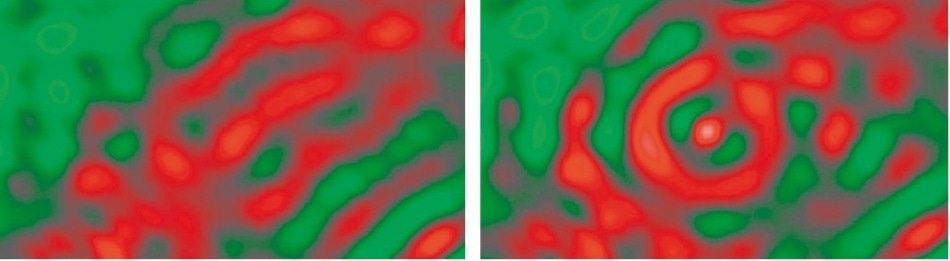
Figure 14. Out-of-plane velocity field after (below) and prior to (above) the impact.
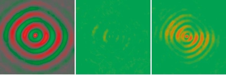
Figure 15. Difference data (Left: out-of-plane, Right: all components, Center: in plane).
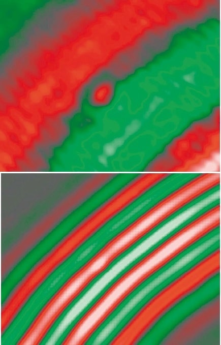
Figure 16. Primary compression waves (left) and flexural waves (right) in the measuring area post impact at 50 kHz (out-of-plane velocity fields).
Summary
The analysis of Lamb wave propagation utilizing scanning laser vibrometry is a favorable tool for detecting damage in panel structures. The measurements enable the assessment of both flexural and compression waves.
The propagation of the total wave field is made apparent, thereby allowing conclusions to be made about the properties of the structure. Systematic errors, which are a common limitation in the use of 1D measuring technology, can be avoided with the implementation of 3D measuring technology which can allow for more accurate results to be acquired.
Defects are presented as distortions in the wave field, mostly in the form of secondary waves generated from mode conversion. As such, the use of this method means that defects can be detected in samples where it would be otherwise impossible using traditional ultrasonic testing, or where it would only be possible with considerably more complexity and cost.

This information has been sourced, reviewed and adapted from materials provided by Polytec.
For more information on this source, please visit Polytec.